2. Suggested solutions weekly assignments - lecture 10

1. In the lecture notes most functions have been implemented to work for finite elements of any order. However, assemble_mass makes use of Ae, which is currently only implemented for \(d=\) 1 and 2. Modify assemble_mass to work for arbitrary orders, by adding a function Ade that returns the element mass matrix of order \(d\). The returned matrix should be a Sympy Matrix including the element length h, as used for A1e and A2e above.

   def Ade(d=1):
       ...
   
   def assemble_mass(xj, d=1):
       N = len(xj)-1
       Ne = N//d
       A = np.zeros((N+1, N+1))
       Ad = Ade(d)
       for elem in range(Ne):
           hj = get_element_length(xj, elem, d=d)
           s0 = local_to_global_map(elem, d=d)
           A[s0, s0] += np.array(Ad.subs(h, hj), dtype=float)
       return A
   

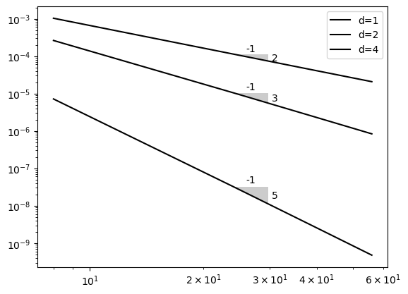
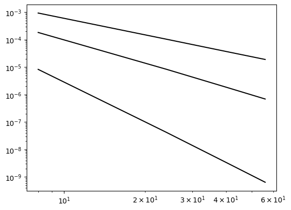
   Run the above example with \(u(x) = \exp(\cos(x))\) and show that \(d=4\) leads to a convergence rate of \(N^{-5}\).

   Hint

   In order to run the example for a range of N that works for both \(d=1, 2\) and \(4\), use \(N \in \{8, 24, 40, 56\}\).

In order to solve this problem and show convergence you can reuse a lot of the code from lecture 10. Only Ade needs to be rewritten in a general manner for any d.

import numpy as np 
import sympy as sp 
import matplotlib.pyplot as plt
from lagrange import Lagrangebasis
from fem import get_element_length, local_to_global_map, assemble_b, fe_evaluate_v
x, h = sp.symbols('x,h')

def Ade(d=1):
    Xj = lambda d: 2*(np.array([sp.Rational(i, d) for i in np.arange(d+1)]))-1 # np.linspace(-1, 1, d+1) only rational
    ll = lambda d: Lagrangebasis(Xj(d))
    qe = lambda l, r, s: sp.integrate(l[r]*l[s], (x, -1, 1))
    A = np.zeros((d+1, d+1), dtype=object)
    l = ll(d)
    for r in range(d+1):
        for s in range(d+1):
            A[r, s] = qe(l, r, s)
    return (h/2)*sp.Matrix(A)

def assemble_mass(xj, d=1):
    N = len(xj)-1
    Ne = N//d
    A = np.zeros((N+1, N+1))
    Ad = Ade(d)
    for elem in range(Ne):
        hj = get_element_length(xj, elem, d=d)
        s0 = local_to_global_map(elem, d=d)
        A[s0, s0] += np.array(Ad.subs(h, hj), dtype=float)
    return A

Reuse some code from lecture 10:

def assemble(u, N, domain=(-1, 1), d=1, xj=None):
    if xj is not None:
        mesh = xj
    else:
        mesh = np.linspace(domain[0], domain[1], N+1)
    A = assemble_mass(mesh, d=d)
    b = assemble_b(u, mesh, d=d)
    return A, b, mesh

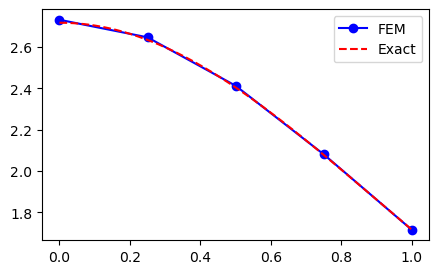
Test for d=1

ue = sp.exp(sp.cos(x))
domain = (0, 1)
A, b, xj = assemble(ue, 4, domain=domain, d=1)
uh = np.linalg.inv(A) @ b
yj = np.linspace(domain[0], domain[1], 200)
plt.figure(figsize=(5, 3))
plt.plot(xj, uh, 'b-o', yj, sp.lambdify(x, ue)(yj), 'r--')
plt.legend(['FEM', 'Exact']);

Run L2-error test for a range of meshes and plot the error

def L2_error(uh, ue, xj, d=1, domain=(-1, 1)):
    yj = np.linspace(domain[0], domain[1], 4*len(xj))
    uhj = fe_evaluate_v(uh, yj, xj, d=d)
    uej = sp.lambdify(x, ue)(yj)
    return np.sqrt(np.trapz((uhj-uej)**2, dx=yj[1]-yj[0]))

error = {}
NN = (8, 24, 40, 56)
for d in (1, 2, 4):
    error[d] = []
    for N in NN:
        A, b, xj = assemble(ue, N, domain=domain, d=d)
        uh = np.linalg.inv(A) @ b
        error[d].append(L2_error(uh, ue, xj, d=d, domain=domain))

from plotslopes import slope_marker
for d in (1, 2, 4):
    plt.loglog(NN, error[d], 'k')
plt.legend(['d=1', 'd=2', 'd=4'])
for d in (1, 2, 4):
    slope_marker((24, error[d][1]), (d+1, -1))

2. Use FEM to approximate the functions in the weekly assignments from lecture 9. That is,

   1. \(u(x) = |x|, \quad x \in [-1, 1]\)

   2. \(u(x) = \exp(\sin(x)), \quad x \in [0, 2]\)

   3. \(u(x) = x^{10}, \quad x \in [0, 1]\)

   4. \(u(x) = \exp(-(x-0.5)^2) - \exp(-0.25) \quad x \in [0, 1]\)

   5. \(u(x) = J_0(x), \quad x \in [0, 100]\)

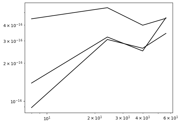
All functions can be approximated with the generic implementation already described above, so there is not much new to do. There are some interesting results though. For example, for \(u(x) = |x|\), the results are exact to machine precision for all \(d\).

error = {}
ue = sp.Abs(x)
domain = (-1, 1)
NN = (8, 24, 40, 56)
for d in (1, 2, 4):
    error[d] = []
    for N in NN:
        A, b, xj = assemble(ue, N, domain=domain, d=d)
        uh = np.linalg.inv(A) @ b
        error[d].append(L2_error(uh, ue, xj, d=d, domain=domain))
for d in (1, 2, 4):
    plt.loglog(NN, error[d], 'k')

The function \(u(x)=x^{10}\) shows results as expected

error = {}
ue = x**10
domain = (0, 2)
NN = (8, 24, 40, 56)
for d in (1, 2, 4):
    error[d] = []
    for N in NN:
        A, b, xj = assemble(ue, N, domain=domain, d=d)
        uh = np.linalg.inv(A) @ b
        error[d].append(L2_error(uh, ue, xj, d=d, domain=domain))
for d in (1, 2, 4):
    plt.loglog(NN, error[d], 'k')

ue = sp.exp(-(x-0.5)**2) - sp.exp(-0.25)
domain = (0, 1)
NN = (8, 24, 40, 56)
for d in (1, 2, 4):
    error[d] = []
    for N in NN:
        A, b, xj = assemble(ue, N, domain=domain, d=d)
        uh = np.linalg.inv(A) @ b
        error[d].append(L2_error(uh, ue, xj, d=d, domain=domain))
for d in (1, 2, 4):
    plt.loglog(NN, error[d], 'k')

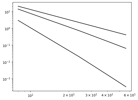
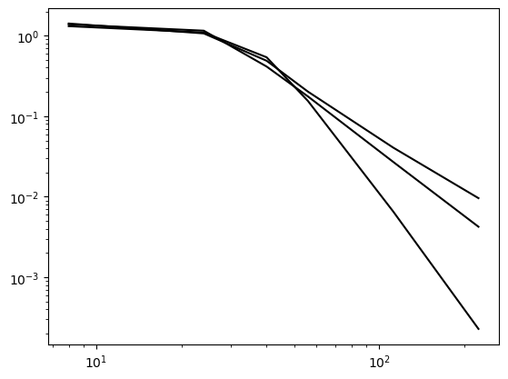
The Bessel function, on the other hand, requires more nodes in order to converge. This is because of the complex shape of the function, that simply cannot be captured with a low number of nodes.

ue = sp.besselj(0, x)
domain = (0, 100)
NN = (8, 24, 40, 56, 112, 224)
for d in (1, 2, 4):
    error[d] = []
    for N in NN:
        A, b, xj = assemble(ue, N, domain=domain, d=d)
        uh = np.linalg.inv(A) @ b
        error[d].append(L2_error(uh, ue, xj, d=d, domain=domain))
for d in (1, 2, 4):
    plt.loglog(NN, error[d], 'k')

For the final assignment, simply try to create code like in lecture 10. To get a working version of FEniCS, see this slide.