Lecture 3

The presentation for lecture 3 is given here.

Vibration equation

The vibration equation can be written as

(3)\[ u^{''} + \omega^2 u = 0, \, t \in (0, T], \, u(0)=I, u'(0) = 0, \]

where \(\omega\) and \(I\) are given constants. This equation is often also referred to as the Helmholtz equation. A simple, recursive, finite difference method for solving the vibration equation is

\[\begin{split} \begin{align*} u^0 &= I\\ u^{1} &= u^0 - \frac{1}{2}\Delta t^2 \omega^2 u^0 \\ u^{n+1} &= 2u^n - u^{n-1} - \Delta t^2 \omega^2 u^{n}, \quad n = 1, 2, \ldots, N_t-1, \end{align*} \end{split}\]

where \(u^n = u(t_n)\) and \(t_n = n \Delta t\).

A recursive solver can easily be created using Numpy:

import numpy as np
import matplotlib.pyplot as plt

def solver(dt, T, w=0.35, I=1):
    """
    Solve Eq. (1)

    Parameters
    ----------
    dt : float
        Time step
    T : float
        End time
    I, w : float, optional
        Model parameters

    Returns
    -------
    t : array_like
        Discrete times (0, dt, 2*dt, ..., T)
    u : array_like
        The solution at discrete times t
    """
    Nt = int(T/dt)
    u = np.zeros(Nt+1)
    t = np.linspace(0, Nt*dt, Nt+1)
    u[0] = I
    u[1] = u[0] - 0.5*dt**2*w**2*u[0]
    for n in range(1, Nt):
        u[n+1] = 2*u[n] - u[n-1] - dt**2*w**2*u[n]
    return t, u

def u_exact(t, w=0.35, I=1):
    """Exact solution of Eq. (1)

    Parameters
    ----------
    t : array_like
        Array of times to compute the solution
    I, w : float, optional
        Model parameters

    Returns
    -------
    ue : array_like
        The solution at times t
    """
    return I*np.cos(w*t)

We now want to compute convergence rates. We will use the \(\ell^2\)-norm computed as

\[E_i = \sqrt{\Delta t_i\sum_{n=0}^{N^{i}_t}(u^n-u_e(t_n))^2},\]

for a given uniform mesh level \(i\). For example, we can use \(N^0_t=8, N_t^{1}=16, N^2_t = 32\), etc., such that \(\Delta t_{1} / \Delta t_2 = 2\) and \(\Delta t_{n-1} / \Delta t_{n} = 2\) for all \(n\). Note that there are \(N_t^{i}\) intervals on level \(i\) and \(N_t^{i}+1\) points.

We assume that the error on the mesh with level \(i\) can be written as

\[E_i = C (\Delta t_i)^r, \]

where \(C\) is a constant. This way, if we have the error on two levels, then we can compute

\[ \frac{E_{i-1}}{E_i} = \frac{ (\Delta t_{i-1})^r}{(\Delta t_{i})^r} = \left( \frac{\Delta t_{i-1}}{ \Delta t_i} \right)^r,\]

and isolate \(r\) by computing

\[ r = \frac{\log {\frac{E_{i-1}}{E_i}}}{\log {\frac{\Delta t_{i-1}}{\Delta t_i}}}. \]

So by computing the error on two different levels we can find the order of the convergence!

Let’s first write a function that computes the \(\ell^2\) error of the solver defined above

def l2_error(dt, T, w=0.35, I=0.3, sol=solver):
    """Compute the l2 error norm of result from `solver`

    Parameters
    ----------
    dt : float
        Time step
    T : float
        End time
    I, w : float, optional
        Model parameters
    sol : callable
        The function that solves Eq. (1)

    Returns
    -------
    float
        The l2 error norm
    """
    t, u = sol(dt, T, w, I)
    ue = u_exact(t, w, I)
    return np.sqrt(dt*np.sum((ue-u)**2))

and then compute the convergence rates

def convergence_rates(m, num_periods=8, w=0.35, I=0.3, sol=solver):
    """
    Return m-1 empirical estimates of the convergence rate
    based on m simulations, where the time step is halved
    for each simulation.

    Parameters
    ----------
    m : int
        The number of mesh levels
    num_periods : int, optional
        Size of domain is num_periods * 2pi / w
    w, I : float, optional
        Model parameters
    sol : callable
        The function that solves Eq. (1)

    Returns
    -------
    array_like
        The m-1 convergence rates
    array_like
        The m errors of the m meshes
    array_like
        The m time steps of the m meshes

    """
    P = 2*np.pi/w
    dt = 1/w # Half the stability limit
    T = P*num_periods
    dt_values, E_values = [], []
    for i in range(m):
        E = l2_error(dt, T, w, I, sol=sol)
        dt_values.append(dt)
        E_values.append(E)
        dt = dt/2
    # Compute m-1 orders that should all be the same
    r = [np.log(E_values[i-1]/E_values[i])/
         np.log(dt_values[i-1]/dt_values[i])
         for i in range(1, m, 1)]
    return r, E_values, dt_values

Test it

convergence_rates(4)

([1.9588768683386768, 2.012815118570204, 2.005023881055473],
 [3.0276628089765527,
  0.7788015566949965,
  0.19297857027753343,
  0.04807693295792429],
 [2.857142857142857,
  1.4285714285714286,
  0.7142857142857143,
  0.35714285714285715])

These last two lists are the errors and timesteps af all the \(m\) levels. We can plot the error as a function of timestep and show that the discretization scheme is second order.

r, E, dt = convergence_rates(5)
plt.loglog(dt, E)
plt.loglog(dt, 10*np.array(dt))
plt.loglog(dt, np.array(dt)**2)
plt.title('Convergence of finite difference method')
plt.legend(['Error', '$\\mathcal{O}(\\Delta t)$', '$\\mathcal{O}(\\Delta t^2)$'])
from plotslopes import slope_marker
slope_marker((dt[1], E[1]), (2,1))
slope_marker((dt[1], 10*dt[1]), (1,1))
slope_marker((dt[1], dt[1]**2), (2,1))

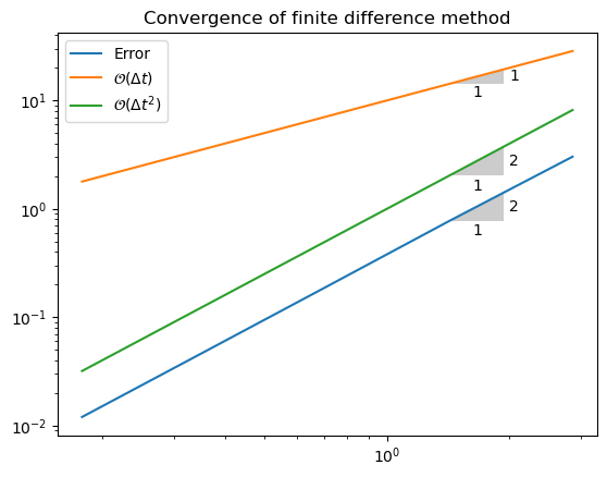
We see that the error has the same slope as \(\Delta t^2\).

We can write a test for the order of accuracy:

def test_order(m, num_periods=5, w=0.5, I=1., sol=solver):
    r, E, dt = convergence_rates(m, num_periods=num_periods, w=w, I=I, sol=sol)
    assert abs(r[-1] - 2) < 1e-2

test_order(5)

Note

The tolerance in test_order is set low \((~10^{-2})\), because this is a limiting order. Normally, the total error gets contributions from many trailing terms in a Taylor series, scaling as \(\Delta t^2, \Delta t^3, \ldots\), and all these errors contribute to the total error that we measure. However, as \(\Delta t \rightarrow 0\) the leading error term dominates and we approach an integer order. If we use more and smaller time steps in convergence_rates, then we can also set the tolerance lower.

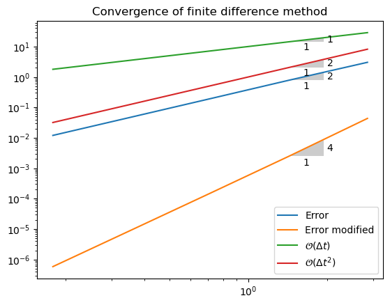
Adjusted solver

def adj_solver(dt, T, w=0.35, I=1):
    """
    Solve Eq. (1)

    Parameters
    ----------
    dt : float
        Time step
    T : float
        End time
    I, w : float, optional
        Model parameters

    Returns
    -------
    t : array_like
        Discrete times (0, dt, 2*dt, ..., T)
    u : array_like
        The solution at discrete times t
    """
    Nt = int(T/dt)
    u = np.zeros(Nt+1)
    t = np.linspace(0, Nt*dt, Nt+1)
    u[0] = I
    u[1] = u[0] - 0.5*dt**2*(w*(1-w**2*dt**2/24))**2*u[0]
    for n in range(1, Nt):
        u[n+1] = 2*u[n] - u[n-1] - dt**2*(w*(1-w**2*dt**2/24))**2*u[n]
    return t, u

r, E, dt = convergence_rates(5, sol=solver)
r2, E2, dt2 = convergence_rates(5, sol=adj_solver)
plt.loglog(dt, E)
plt.loglog(dt2, E2)
plt.loglog(dt, 10*np.array(dt))
plt.loglog(dt, np.array(dt)**2)
plt.title('Convergence of finite difference method')
plt.legend(['Error', 'Error modified', '$\\mathcal{O}(\\Delta t)$', '$\\mathcal{O}(\\Delta t^2)$'])
from plotslopes import slope_marker
slope_marker((dt[1], E[1]), (2,1))
slope_marker((dt2[1], E2[1]), (4,1))
slope_marker((dt[1], 10*dt[1]), (1,1))
slope_marker((dt[1], dt[1]**2), (2,1))

Method of manufactured solutions

We will now use the method of manufactured solutions (MMS) to verify that the solver works. This is a method that will be used a lot throughout the course.

With the MMS we first need to assume that we know the solution. For example, we assume that the solution is

\[ u(t) = t^2. \]

It is important that the solution satisfies the boundary conditions: \(u(0)=0\) and \(u'(0)=0\). However, if we plug the solution into the Helmholtz equation, we do not get a zero right hand side

\[ u''(t) + \omega^2 u(t) = 2 + \omega^2 t^2 \ne 0. \]

So we need to use a nonzero right hand side of Eq. (3):

\[ u''(t) + \omega^2 u(t) = f(t), \]

where for the chosen manufactured solution \(f(t) = 2 + \omega^2 t^2\).

The point with the manufactured solution is that is satisfies the equation above, which is the same as the original, but with an additional source term. Source terms are not differentiated, so they do not pose any additional difficulty.

Assume now that the solution is

\[ u(t) = t^4. \]

Initial conditions are still ok. Now the equation that satisfies this manufactured solution becomes

\[ u'' + \omega^2 u = 12 t^2 + \omega^2 t^4, \]

so \(f(t) = 12 t^2 + \omega^2 t^4\). Since the solution is a fourth order polynomial, the second order numerical method will not be exact, but it will converge to the right solution.

For the MMS we need to create a solver such that

\[ u^{''} + \omega^2 u = f, \, t \in (0, T], \, u(0)=I, u'(0) = 0, \]

The recursive method becomes

\[\begin{split} \begin{align*} u^0 &= I\\ u^{1} &= u^0 - \frac{1}{2}\Delta t^2 \omega^2 u^0 + \frac{\Delta}{2} t^2 f^0 \\ u^{n+1} &= 2u^n - u^{n-1} - \Delta t^2 \omega^2 u^{n} + \Delta t^2 f^n, \quad n = 1, 2, \ldots, N_t-1, \end{align*} \end{split}\]

And the numerical solution obtained can now be compared, using the \(\ell^2\) error norm, with the manufactured solution!