Lecture 10 - Function approximation by the finite element method#
The finite element method#
We have seen that a function \(u(x)\) can be approximated as
And we have seen how the least squares, Galerkin and collocation methods can be used to find the unknown \(\boldsymbol{\hat{u}} = (\hat{u}_j)_{j=0}^N\). Up until now we have used global basis functions \(\psi_j(x)\) defined on the entire domain \(\Omega\).
The global aspect of the basis functions is an advantage when it comes to both accuracy and efficiency. However, we are not always interested in solving equations on a simple line interval, or a rectangle for two dimensions. Normally we are more interested in domains that contain some physical obstructions, like Fig. 1.
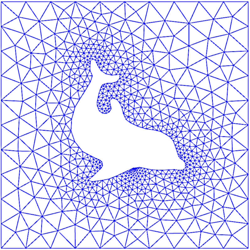
Fig. 1 Example of finite element mesh.#
For such domains, like the dolfin mesh, it is not possible to use basis functions that are defined everywhere. It is also very difficult, if not impossible, to use finite difference methods. Just imagine, how would you implement a Laplacian, like
on a 2D dolfin mesh?
The finite element method, on the other hand, is designed to work on such triangulated and unstructured meshes in complex domains. But in order to present the method it makes sense to first stick to simple one-dimensional domains also here.
The finite element method (FEM) starts by splitting the domain \(\Omega\) into \(N_e\) smaller, non-overlapping, subdomains \(\Omega^{(e)}\), such that
For example, the domain \(\Omega = [0, 5]\) can be split up into 5 smaller subdomains \(\Omega^{(e)} = [e, e+1], e \in (0, 1, 2, 3, 4)\) using 6 uniformly distributed nodes:
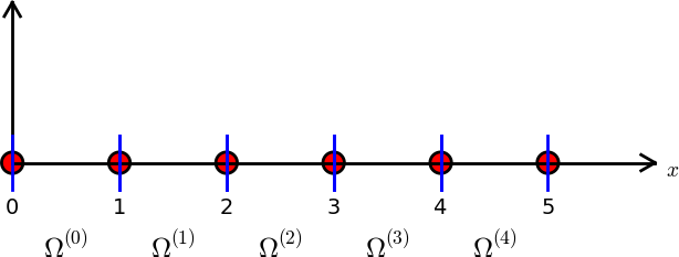
Fig. 2 Finite element mesh with 5 elements and 6 nodes.#
These smaller subdomains are now referred to as elements. Note that an element in Fig. 2 is located in between two blue vertical bars.
The mesh seen in Fig. 2 is the simplest possible FEM mesh, where each element contains 2 nodes. These elements can at best make use of linear polynomials as basis functions since there are only 2 nodes in each element.
A slightly more complicated mesh is shown in Fig. 3, which is non-uniform and contains only 2 elements and 5 nodes. Each of the elements contains 3 nodes, and as such these elements can make use of second order polynomials.
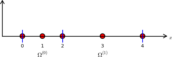
Fig. 3 Finite element mesh with 2 elements and 5 nodes.#
The dolfin mesh of course is a more complicated triangulation, where every triangle represents an element. It is also quite common to use rectangles in 2D. For 3D problems a finite element is usually in the shape of a tetrahedron.
Finite element basis functions#
The FEM makes use of local basis functions that are only non-zero on some of the elements. Furthermore, the basis functions that we will make use of in this class are continuous piecewise polynomials. In the simplest possible form, this means that the basis functions are piecewise linear. For example, for the mesh in Fig. 2 two of the 6 basis functions will be as shown below:
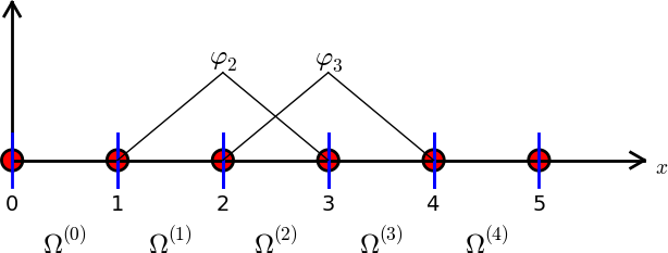
Fig. 4 Finite element mesh with 5 elements, 6 nodes and two of the 6 basis functions.#
The finite element method is a variational method. As such we can define the problem of approximating functions exactly the same way as we did for the global approach. Assume that we want to use the finite element method to find an approximation to \(u(x)\) in \(\Omega=[0, 5]\). If we use the mesh in Fig. 2 we get a function space \(V_N = \text{span}\{\psi_j\}_{j=0}^5\), where \(\psi_j(x)\) are the 6 piecewise linear functions that are 1 on node \(j\), zero on all the other nodes and linear in between. We then attempt to find \(u_N \in V_N\) such that
It is also possible to use the least squares method, but this is very rare. So for the finite element method we will focus on the Galerkin method with continuous piecewise polynomial basis functions.
Note
The Galerkin formulation is the same whether you use a global approach with Legendre polynomials or a local FEM with piecewise polynomials. The difference lies all in the function spaces and the choice of basis.
Note
Other than the fact that the basis functions are piecewise polynomials with only local support, there is nothing new from the previous chapters. It is only much more complicated to work with local functions than global and it requires much more effort to implement.
In this class we will use Lagrange polynomials as basis functions for the finite element method. But not global Lagrange polynomials, only local; local to elements. In this way it is similar to using Lagrange polynomials for interpolation on a finite difference grid.
Each element in Fig. 2 contains 2 nodes. These nodes will locally be denoted as \((x^0, x^1)\) no matter which element we are in, and the Lagrange formula is then
There are exactly two linear Lagrange polynomials on each element, and these are locally computed as
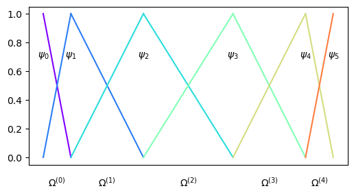
We can plot all these basis functions with one color for each basis function \(\psi_j(x)\)
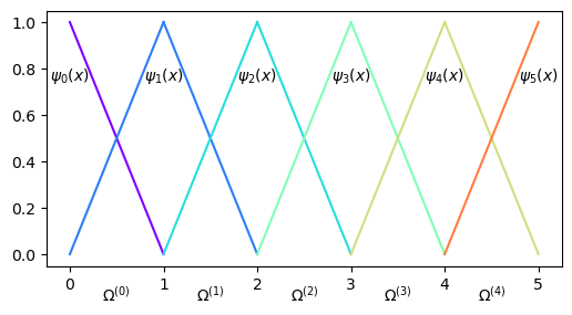
So all the internal basis functions, i.e., \(\{\psi_j(x)\}_{j=1}^{4}\), are nonzero in two elements each and zero elsewhere. The two boundary basis functions \(\psi_0(x)\) and \(\psi_5(x)\) are only nonzero on one element each.
Since we are using Lagrange polynomials all basis functions satisfy
for all mesh points \((x_i)_{i=0}^N\). This applies not only for uniform meshes, but for any collection of mesh points. Assume that the mesh uses Chebyshev points instead. This is no problem for the elements of the Lagrange polynomials:
The flexibility when it comes to mesh is one of the major advantages of the finite element method, which can be used with any kind of unstructured mesh.
For any 1D mesh we get the piecewise linear Lagrange basis functions
for \(j = 0, 1, \ldots, N\). Note that \(x_{-1}\) and \(x_{N+1}\) are undefined, but this is irrelevant because the basis functions will not be used outside the domain \(\Omega = [x_0, x_N]\).
A function space for the piecewise linear polynomials can be defined as \(V_N = \text{span}\{\psi_j\}_{j=0}^N\) and with the Galerkin method we approximate any function \(u(x)\) by looking for \(u_N \in V_N\) such that
In other words, we need to solve the follow linear algebra problem
This is identical to the Galerkin problem already presented in lecture 8. Again, the only difference is the choice of function spaces and basis.
Unfortunately, the finite element mass matrix \(A = (a_{ij})_{i,j=0}^N\), with
is not diagonal, because the basis functions are not orthogonal. However, since the basis functions are local the matrix will still be highly sparse.
Since the basis functions are piecewise polynomials and only some of the basis fucntions are nonzero on each element, we usually assemble the matrix elementwise as
Here we will identify
as the element mass matrix, and note that this matrix is still of shape \((N+1) \times (N+1)\), even though for any given element it will only consist of a few nonzero items. The full mass matrix can now be written as
The element mass matrix \(A^{(e)}=(a^{(e)}_{ij})_{i,j=0}^N\) is very sparse since it only has nonzero items for indices \(i, j\) corresponding to nonzero basis functions in the element \(e\). Hence it makes sense to reduce its size. If there are \(d+1\) nonzero basis functions on each element, then there can be at most \((d+1)^2\) nonzero combinations of \(i\) and \(j\) in \((\psi_i, \psi_j)\) and the element matrix \(\tilde{A}^{(e)}\) can as such be represented as a dense \((d+1)\times (d+1)\) matrix
where
and \(q(e,r)\) is a mapping function that maps a local index \(r\) on the global element \(e\) to a global index. For a structured mesh like Fig. 2 and Fig. 3, and elements with \(d+1\) nodes in each, we get the mapping
Note
The matrix \(\tilde{A}^{(e)}\) contains the same nonzero items as \(A^{(e)}\), but \(\tilde{A}^{(e)}\in \mathbb{R}^{(d+1) \times (d+1)}\) is dense, whereas \(A^{(e)} \in \mathbb{R}^{(N+1)\times (N+1)}\) is highly sparse. The small matrices in Fig. 5 represent \(\tilde{A}^{(e)}\).
In order to use the local (and small) element matrices \(\tilde{A}^{(e)}\) we assemble for each element into the global matrix \(A\) as
This process, which is termed finite element assembly, can be illustrated as shown below, where 4 small element matrices \(\tilde{A}^{(e)}\) of shape \(2 \times 2\) are inserted into the global matrix \(A\) of shape \(5 \times 5\). For this linear case \(d=1\). Note that there is overlap between the 4 element matrices in the global \(A\), because all the internal (linear) basis functions are nonzero in 2 elements each.
Fig. 5 Finite element assembly of the local element matrices \(\tilde{A}^{(e)}\) into the global matrix \(A\). Note the mapping of local to global indices above the matrix \(A\).#
Mapping to reference domain#
In assembling the matrix \(A\) we need to compute the element matrix \(\tilde{A}^{(e)}\) many times. Is this really necessary? The integrals
differ only in the domain, whereas the shape of the basis functions are the same regardless of domain. The piecewise linear basis functions are always straight lines from one in one node to zero in the other:
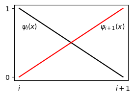
So the basis functions always look the same regardless of domain, regardless of what \(x_i\) and \(x_{i+1}\) are. Hence it should be possible to perform the integration once, in a reference domain, and then reuse this result for all elements. This can be achieved by mapping to a reference domain, which has already been used for both Legendre and Chebyshev polynomials, but for slightly different reasons. For those two, we needed to map because the polynomials and weight functions were only defined on a reference domain.
We will now use this linear (affine) mapping and the same reference domain \([-1, 1]\) as the Chebyshev/Legendre polynomials. In this domain the mapping from physical coordinate \(x \in \Omega^{(e)} = [x_{q(e,0)}, x_{q(e, d)}] = [x_L, x_R]\) to computational (or reference) coordinate \(X \in [-1, 1]\) can be written as
Note that \(x_L\) and \(x_R\) are the left and right boundary points of the domain \(\Omega^{(e)}\). If we introduce the center of the element as \(x_m = (x_L+x_R)/2\) and the element length \(h = x_R-x_L\), then the mapping can be written simply as
The basis functions are then mapped such that
where the Lagrange basis functions
Here \((X_s)_{s=0}^d\) are the \(d+1\) nodes in reference coordinates. For linear elements, with \(d=1\), \((X_0, X_1) = (-1, 1)\) and for quadratic, with \(d=2\), \((X_0, X_1, X_2) = (-1, 0, 1)\). In general,
We get the reference basis functions for linear elements
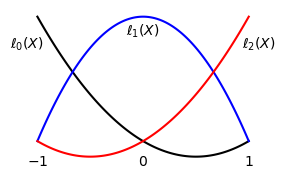
and for quadratic
The quadratic basis functions are shown below in the reference domain.
The mapping should now be used in a change of variables for the inner product:
where \(dx/dX = h/2\), such that for any element, regardless of order \(d\), we can compute the elements of the element matrix as
Hence, instead of computing the element matrix for linear polynomials as
we can simply use
The four integrals can be evaluated once and for all, and reused for all elements and any mesh, uniform or nonuniform, simply by scaling the matrix with the element length \(h\). We can also compute this element matrix easily using Sympy
h = sp.Symbol('h')
l = Lagrangebasis([-1, 1])
ae = lambda r, s: sp.integrate(l[r]*l[s], (x, -1, 1))
A1e = h/2*sp.Matrix([[ae(0, 0), ae(0, 1)],[ae(1, 0), ae(1, 1)]])
A1e
Using quadratic elements, we get
l2 = Lagrangebasis([-1, 0, 1])
a2e = lambda r, s: sp.integrate(l2[r]*l2[s], (x, -1, 1))
A2e = h/2*sp.Matrix([[a2e(0, 0), a2e(0, 1), a2e(0, 2)],
                     [a2e(1, 0), a2e(1, 1), a2e(1, 2)],
                     [a2e(2, 0), a2e(2, 1), a2e(2, 2)]])
A2e
Note
The mass matrix and all the element mass matrices are always symmetrical, meaning that \(a_{ij} = a_{ji}\) and \(a_{ij}^{(e)} = a_{ji}^{(e)}\) for all \(i, j\). This means that it is unnecessary to compute both \(a^{(e)}_{ij}\) and \(a^{(e)}_{ji}\) as we have done above. It is sufficient to compute \(a^{(e)}_{ij}\) by integration, and then you can simply set \(a^{(e)}_{ji}=a^{(e)}_{ij}\).
Since we know how to compute the element matrix, we also know how to compute the full mass matrix. The following function assemble_mass sums over all elements and adds the contribution from each to the matrix \(A\). We also create a few helper functions get_element_boundaries and get_element_length with obvious purpose and the local to global map \(q(e, r)\). Note that if \(r\) is not provided, then local_to_global_map returns a slice representing the global indices \(\{q(e, r)\}_{r=0}^{d}\).
Ae = [A1e, A2e] # previously computed

def get_element_boundaries(xj, e, d=1):
    return xj[d*e], xj[d*(e+1)]

def get_element_length(xj, e, d=1):
    xL, xR = get_element_boundaries(xj, e, d=d)
    return xR-xL

def local_to_global_map(e, r=None, d=1): # q(e, r)
    if r is None:
        return slice(d*e, d*e+d+1)
    return d*e+r

def assemble_mass(xj, d=1):
    N = len(xj)-1
    Ne = N//d
    A = np.zeros((N+1, N+1))
    for elem in range(Ne):
        hj = get_element_length(xj, elem, d=d)
        s0 = local_to_global_map(elem, d=d)
        A[s0, s0] += np.array(Ae[d-1].subs(h, hj), dtype=float)
    return A
N = 4
xj = np.linspace(1, 2, N+1)
A = assemble_mass(xj, d=1)
print(A)
[[0.08333333 0.04166667 0.         0.         0.        ]
 [0.04166667 0.16666667 0.04166667 0.         0.        ]
 [0.         0.04166667 0.16666667 0.04166667 0.        ]
 [0.         0.         0.04166667 0.16666667 0.04166667]
 [0.         0.         0.         0.04166667 0.08333333]]
The mass matrix for second order polynomials on a uniform mesh can be computed as
N = 8
xj = np.linspace(1, 2, N+1)
A = assemble_mass(xj, d=2)
We can plot the sparsity pattern of the matrix A using plt.spy. This function plots a square for all the nonzero items of A, and nothing where it is zero.
plt.figure(figsize=(3, 3))
plt.spy(A, markersize=5);
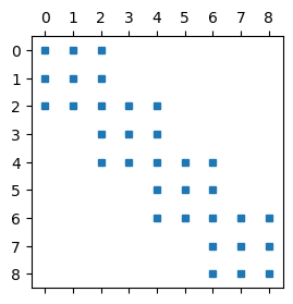
Note that there is a big difference between nodes on the boundaries between elements and internal nodes. The rows in \(A\) above corresponding to internal nodes have only three nonzero items, whereas the nodes on element boundaries have 5. This is because the basis functions on the element boundaries belong to two elements, whereas the internal nodes only belong to one.
Note
For the matrices computed above we have used a uniform mesh such that \(h\) is constant. A non-uniform mesh needs to take into account the different element sizes \(h\), but this is only a matter of scaling the element matrices \(\tilde{A}^{(e)}\). assemble_mass works also for a non-uniform mesh, because the size of each element is taken into account.
Finite element assembly of a vector#
We now know how to compute the mass matrix in (39), but we also need the right hand side \(b_i = (u, \psi_i), i = 0, 1, \ldots, N\). This inner product can also be evaluated elementwise, and mapped just like the mass matrix. We define the element vector similarly as the element matrix (\(A^{(e)}\))
and note that \(\boldsymbol{b}^{(e)} = (b^{(e)}_i)_{i=0}^N \in \mathbb{R}^{N+1}\) is a very sparse vector since \(b_i^{(e)}\) only is nonzero if \(i\) is a node in the element \(e\). Hence, it also makes sense to define a dense vector \(\boldsymbol{\tilde{b}}^{(e)} \in \mathbb{R}^{d+1}\) (similar to \(\tilde{A}^{(e)}\)) containing only the nonzero items of \(\boldsymbol{b}^{(e)}\)
With a mapping to the reference space we get
We can create a function assemble_b to do this assembly for any order \(d\) and a generic Sympy function \(u(x)\). To this end we also create some helper functions map_true_domain and map_reference_domain, that return \(x(X)\) and \(X(x)\), respectively. The function map_u_true_domain returns \(\tilde{u}(X) = u(x(X))\).
from scipy.integrate import quad

def map_true_domain(xj, e, d=1, x=x): # return x(X)
    xL, xR = get_element_boundaries(xj, e, d=d)
    hj = get_element_length(xj, e, d=d)
    return (xL+xR)/2+hj*x/2

def map_reference_domain(xj, e, d=1, x=x): # return X(x)
    xL, xR = get_element_boundaries(xj, e, d=d)
    hj = get_element_length(xj, e, d=d)
    return (2*x-(xL+xR))/hj

def map_u_true_domain(u, xj, e, d=1, x=x): # return u(x(X))
    return u.subs(x, map_true_domain(xj, e, d=d, x=x))

def assemble_b(u, xj, d=1):
    l = Lagrangebasis(np.linspace(-1, 1, d+1), sympy=False)
    N = len(xj)-1
    Ne = N//d
    b = np.zeros(N+1)
    for elem in range(Ne):
        hj = get_element_length(xj, elem, d=d)
        us = sp.lambdify(x, map_u_true_domain(u, xj, elem, d=d))
        integ = lambda xj, r: us(xj)*l[r](xj)
        for r in range(d+1):
            b[d*elem+r] += hj/2*quad(integ, -1, 1, args=(r,))[0]
    return b
Lets use these basis functions for the Galerkin method in order to approximate \(u(x) = 10(x-1)^2-1, x \in [1, 2]\). We use first a uniform mesh, assemble the mass matrix \(A\) and the vector \(\boldsymbol{b}\) and then solve the linear algebra system:
def assemble(u, N, domain=(-1, 1), d=1, xj=None):
    if xj is not None:
        mesh = xj
    else:
        mesh = np.linspace(domain[0], domain[1], N+1)

    A = assemble_mass(mesh, d=d)
    b = assemble_b(u, mesh, d=d)
    return A, b

# Create uniform mesh
N = 4
xj = np.linspace(1, 2, N+1)

A, b = assemble(10*(x-1)**2-1, N, d=1, xj=xj)
uh = np.linalg.inv(A) @ b
yj = np.linspace(1, 2, 1000)
plt.figure(figsize=(5, 3))
plt.plot(xj, uh, 'b-o', yj, 10*(yj-1)**2-1, 'r--')
plt.legend(['FEM', 'Exact']);
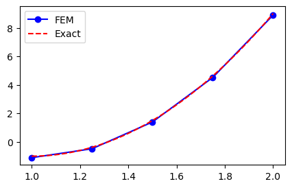
Not bad, but clearly not exact since the FEM solution is piecewise linear between the 5 mesh points. How about second order? We have implemented assemble to use higher order, so it should be straight forward. Just to check that a non-uniform mesh works as well we create a mesh where the element boundaries in the physical domain \([1, 2]\) are computed as
and then the internal nodes are computed as
# Create nonuniform mesh where all internal nodes are in
# the center of the elements
N = 6
xj = np.zeros(N+1)
xj[::2] = 1 + (np.cos(np.arange(N//2+1)*np.pi*2/N)[::-1] + 1)/2
xj[1::2] = 0.5*(xj[:-1:2]+xj[2::2])
A, b = assemble(10*(x-1)**2-1, N, d=2, xj=xj)
uh = np.linalg.inv(A) @ b
yj = np.linspace(1, 2, 1000)
plt.figure(figsize=(5, 3))
plt.plot(xj, uh, '-bo', yj, 10*(yj-1)**2-1, 'r--')
plt.legend(['FEM 2nd order', 'Exact']);
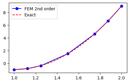
But what happened here? The results still look like piecewise linear polynomials and it looks no better than before. The problem now is not accuracy of the FEM approximation, though, it has more to do with postprocessing and finite element evaluation. We compute and plot the finite element solution \((\hat{u}_j)_{j=0}^N\), but then matplotlib simply fills in the gaps between the points with linear profiles. The correct approach would be to evaluate the finite element function
in between the mesh points.
Finite element evaluation#
The finite element solution differs from the finite difference solution in that the solution is automatically defined everywhere within the domain. The finite difference solution is only defined in mesh points and requires interpolation. With FEM we need to evaluate (44). To this end note that the point \(x\) is either
at a mesh point \(x_i\), in which case \(u_N(x_i) = \hat{u}_i\).
in between mesh points and inside one and only one element.
In case of the second event we can evaluate \(u_N(x)\) by mapping to the reference domain simply as
So we only need to figure out which element the point \(x\) is in and then simply evaluate the nonzero polynomials on that element only. To this end it does not hurt to remind ourselves of formulas that we can use for our structured (uniform) grids:
Mesh |
Formula |
|---|---|
domain |
\(\Omega = [a, b]\) |
Reference domain |
\(\Omega^{(e)} = [-1, 1]\) |
Order of polynomials |
\(d\) |
Number of nodes in physical mesh |
\(N+1\) |
Number of elements in mesh |
\(N_e = N / d\) |
Element index |
\(e \quad \in \{0, 1, \ldots, N_e-1\}\) |
physical mesh points uniform grid |
\(x_i = a + \frac{i h}{N}, \quad i = 0, 1, \ldots, N\) |
physical mesh points any grid |
\(x_i \quad i = 0, 1, \ldots, N\) |
element boundaries |
\(x_i \quad i = 0, d, \ldots, N/d\) |
Local to global mapping q(e, r) |
\(q(e, r) = d e + r, \quad r = 0, 1, \ldots, d\) |
Map to true coordinate x(X) |
\(x = \frac{1}{2}(x_L+x_R) + \frac{1}{2}(x_R-x_L)X\) |
Physical boundary of element \(e\) |
\([x_L, x_R], \quad x_L = x_{q(e, 0)}, x_R = x_{q(e, d)}\) |
Element length |
\(h = x_R-x_L\) |
Reference mesh points |
\(X_r = -1 + \frac{2r}{d}, \quad r = 0, 1, \ldots, d\) |
An implementation of finite element evaluation for a single point is shown below:
def fe_evaluate(uh, p, xj, d=1):
    l = Lagrangebasis(np.linspace(-1, 1, d+1), sympy=False)
    elem = max(0, np.argmax(p <= xj[::d])-1) # find element containing p
    Xx = map_reference_domain(xj, elem, d=d, x=p)
    return Lagrangefunction(uh[d*elem:d*(elem+1)+1], l)(Xx)
Note
We find the element that the point \(p\) belongs to by finding the smallest index in the element boundary mesh \((x_i), \, i = 0, d, \ldots, N/d\), where \(x_i \le p\).
We can now evaluate the finite element function uh computed above with second order accuracy. For example for point \(x=1.2\):
fe_evaluate(uh, 1.2, xj, d=2), 10*(1.2-1)**2-1
(-0.600000000000000, -0.6000000000000002)
The solution is exact to machine precision because the interpolated function is a second order polynomial.
A disadvantage is that fe_evaluate only works for single points. For efficiency we should vectorize it
def fe_evaluate_v(uh, pv, xj, d=1):
    l = Lagrangebasis(np.linspace(-1, 1, d+1), sympy=False)
    elem = (np.argmax((pv <= xj[::d, None]), axis=0)-1).clip(min=0) # find elements containing pv
    xL = xj[:-1:d] # All left element boundaries
    xR = xj[d::d]  # All right element boundaries
    xm = (xL+xR)/2 # middle of all elements
    hj = (xR-xL)   # length of all elements
    Xx = 2*(pv-xm[elem])/hj[elem] # map pv to reference space all elements
    dofs = np.array([uh[e*d+np.arange(d+1)] for e in elem], dtype=float)
    V = np.array([lr(Xx) for lr in l], dtype=float) # All basis functions evaluated for all points
    return np.sum(dofs * V.T, axis=1)
Check the vectorized version by evaluating two points and compare with exact solution.
from IPython.display import display
display(fe_evaluate_v(uh, np.array([1.2, 1.3]), xj, d=2))
display((10*(1.2-1)**2-1, 10*(1.3-1)**2-1))
array([-0.6, -0.1])
(-0.6000000000000002, -0.09999999999999976)
Lets try the more difficult function
that required 20 Legendre or Chebyshev coefficients for full machine precision. Loop over a range of mesh sizes and compute both with linear and quadratic basis functions. When finished compute the \(L^2\) error norm using a numerical integral with 4 times as many points as the numerical solution.
def L2_error(uh, ue, xj, d=1):
    yj = np.linspace(-1, 1, 4*len(xj))
    uhj = fe_evaluate_v(uh, yj, xj, d=d)
    uej = ue(yj)
    return np.sqrt(np.trapz((uhj-uej)**2, dx=yj[1]-yj[0]))

u = sp.exp(sp.cos(x))
ue = sp.lambdify(x, u)
err = []
err2 = []
for n in range(2, 30, 4):
    N = 2*n
    xj = np.linspace(-1, 1, N+1)
    A, b = assemble(u, N, (-1, 1), 1)
    uh = np.linalg.inv(A) @ b
    A2, b2 = assemble(u, N, (-1, 1), 2)
    uh2 = np.linalg.inv(A2) @ b2
    err.append(L2_error(uh, ue, xj, 1))
    err2.append(L2_error(uh2, ue, xj, 2))
/var/folders/ql/nly59sfj4dd3spkth6lk0kjw0000gn/T/ipykernel_55518/387443513.py:5: DeprecationWarning: `trapz` is deprecated. Use `trapezoid` instead, or one of the numerical integration functions in `scipy.integrate`.
  return np.sqrt(np.trapz((uhj-uej)**2, dx=yj[1]-yj[0]))
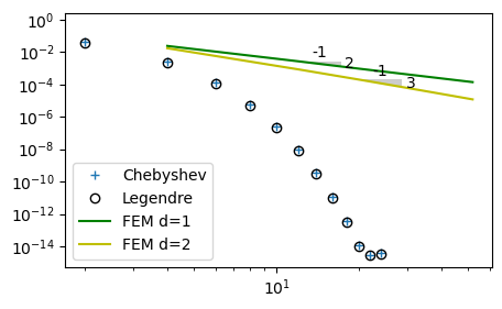
The FEM approximation using linear polynomials should be second order accurate, because the linear \(\ell_0\) and \(\ell_1\) have Taylor expansions where the first neglected term is proportional to \(\Delta x^2\). Similarly, the FEM approximation using second order polynomials should be third order. As stated in lecture 9 the Chebyshev and Legendre approximations have spectral accuracy, which is faster than any finite order. This is easy to illustrate. In the figure below we plot the \(L^2\) errors of the Legendre/Chebyshev approximations as well as the FEM. Note how the spectral methods accelerate towards machine precision, whereas the error for FEM disappears at a rate proportional to \(N^{-2}\) and \(N^{-3}\). The global approximation using \(N=8\) achieves better accuracy than local quadratic elements with \(N=52\).
err_cl = np.load('./err_u.npy')
plt.figure(figsize=(5, 3))
plt.loglog(np.arange(0, 25, 2), err_cl[0], '+',
           np.arange(0, 25, 2), err_cl[1], 'ko',
           np.arange(2, 30, 4)*2, err, 'g',
           np.arange(2, 30, 4)*2, err2, 'y',
           fillstyle='none')
from plotslopes import slope_marker
slope_marker((12, err[1]), (2, -1))
slope_marker((20, err2[2]), (3, -1))
plt.legend(['Chebyshev', 'Legendre', 'FEM d=1', 'FEM d=2']);
Weekly assignments#
In the lecture notes above most functions have been implemented to work for finite elements of any order. However, assemble_mass makes use of
Ae, which is currently only implemented for \(d=\) 1 and 2. Modifyassemble_massto work for arbitrary orders, by adding a functionAdethat returns the element mass matrix of order \(d\). The returned matrix should be a Sympy Matrix including the element lengthh, as used forA1eandA2eabove.def Ade(d=1): ... def assemble_mass(xj, d=1): N = len(xj)-1 Ne = N//d A = np.zeros((N+1, N+1)) Ad = Ade(d) for elem in range(Ne): hj = get_element_length(xj, elem, d=d) s0 = local_to_global_map(elem, d=d) A[s0, s0] += np.array(Ad.subs(h, hj), dtype=float) return A
Run the above example with \(u(x) = \exp(\cos(x))\) and show that \(d=4\) leads to a convergence rate of \(N^{-5}\).
Hint
In order to run the example for a range of
Nthat works for both \(d=1, 2\) and \(4\), use \(N \in \{8, 24, 40, 56\}\).Use FEM to approximate the functions in the weekly assignments from lecture 9
Use FEniCS to approximate the same functions as in assignment 2. See lecture 10.