Lecture 12

Solving PDEs with the finite element method

The procedure for solving differential equations with the finite element method is much the same as for global basis functions. However

• Basis functions are local

• We always use reference elements

• Matrices are assembled elementwise

• We will only use polynomials for basis functions

• PDEs are normally not solved using tensor products in multiple dimensions

As always we work with a function space \(V_N = \text{span}\{\psi_{j}\}_{j=0}^N\) and approximations (in 1D)

\[ u_N(x) = \sum_{j=0}^N \hat{u}_j \psi_j(x). \]

The basis functions \(\psi_i\) for the FEM were discussed in lecture 10, where we also discussed finite element assembly of the mass matrix

\[ a_{ij} = (\psi_j, \psi_i) = \sum_{e=0}^{N_e-1} \int_{\Omega^{(e)}} \psi_j \psi_i d\Omega. \]

In this lecture we move one step further and use the FEM to solve differential equations. Exactly like in lecture 11 this means that we want to find \(u_N \in V_N\) such that

(57)\[ (\mathcal{R}_N, v) = 0, \quad \forall \, v \in V_N, \]

where \(\mathcal{R}_N = \mathcal{L}(u_N)-f\) is a residual and \(\mathcal{L}(u)\) is some mathematical operator acting on \(u\). See lecture 11.

The finite element method as defined here is a Galerkin method, which is also classified as a method of weighted residuals (MWR). We remember from lecture 11 that for MWR the test space in Eq. (57) may also take other forms, but here we will focus on Galerkin.

We will start this lecture by considering Poisson’s equation

\[ u'' = f, \quad x \in (0, L), \, u(0) = a, u(L) = b, \]

using piecewise linear polynomials as basis functions. The variational Galerkin form is now to find \(u_N \in V_N\) such that

\[ (u_N'', v) = (f, v), \quad \forall \, v \in V_N, \]

which is modified using integration by parts into

\[ (u_N', v') = -(f, v) + [u_N'v]_{x=0}^{x=L}, \quad \forall \, v \in V_N. \]

Inserting for \(u_N\) and \(v=\psi_i\) we get the linear algebra problem

(58)\[ \sum_{j=0}^N(\psi'_j, \psi'_i) \hat{u}_j = -(f, \psi_i) + \left(u'_N(L)\psi_i(L) - u'_N(0)\psi_i(0)\right). \]

The boundary term \(u'_N(L)\psi_i(L) - u'_N(0)\psi_i(0)\) can be used to specify Neumann boundary conditions, and we will get back to that. But first we consider only Dirichlet conditions. How can these be implemented? The boundary terms contain only the derivatives \(u'_N\) and not \(u(0)\) or u(L), so this cannot be used. However, remember that the finite element solution is using Lagrange polynomials that are such that

\[ \psi_j(x_i) = \delta_{ij}. \]

Hence

\[ u(0) = u_N(x_0) = \sum_{j=0}^N \hat{u}_j \psi_j(x_0) = \psi_0(x_0) \hat{u}_0 = \hat{u}_0 = a, \]

and

\[ u(L) = u_N(x_N) = \sum_{j=0}^N \hat{u}_j \psi_j(x_N) = \psi_N(x_N) \hat{u}_N = \hat{u}_N = b. \]

So the two expansion coefficients \(\hat{u}_0\) and \(\hat{u}_N\) are known. That means that we only need to solve (58) for \(i = 1, 2, \ldots, N-1\). And the boundary terms \(u'_N(L)\psi_i(L) - u'_N(0)\psi_i(0)\) are only (possibly) nonzero for \(i=0\) or \(i=N\), because only \(\psi_0\) and \(\psi_N\) are nonzero at the edges (at \(x_0\) and \(x_N\)). That is, the only nonzero terms are \(u'_N(L)\psi_N(L) - u'_N(0)\psi_0(0)\) and as such the boundary terms will only enter the assembled equations (58) for the unknowns \(i=0\) and \(i=N\). But these are not unknown, so with Dirichlet boundary conditions we can simply neglect the boundary terms! We will get back to these boundary term for Neumann boundary conditions though.

Note

Remember that in the linear algebra problem (58) each row represents a linear equation. And \(i=0\) represents the equation for the left boundary, whereas \(i=N\) represents the equation for the right boundary. Since Dirichlet boundary conditions dictate that \(\hat{u}_0=a\) and \(\hat{u}_N=b\), we ident the two rows and put \(a\) and \(b\) in the right hand side vector.

\[\begin{split} \begin{bmatrix} 1 & 0 & 0 & \cdots & 0 \\ s_{10} & s_{11}& s_{12} & \cdots & s_{1N} \\ \vdots & \vdots & \vdots & \ddots & \cdots \\ s_{N-1, 0} & s_{N-1, 1}& s_{N-1, 2}& \cdots & s_{N-1,N} \\ 0 & \cdots & 0 & 0 & 1 \end{bmatrix} \begin{bmatrix} \hat{u}_0 \\ \hat{u}_1 \\ \vdots \\ \hat{u}_{N-1} \\ \hat{u}_N \end{bmatrix} = \begin{bmatrix} a \\ f_1 \\ \vdots \\ f_{N-1} \\ b \end{bmatrix} \end{split}\]

To solve (58), the right hand side is treated exactly as in lecture 10, whereas we need to assemble the stiffness matrix

\[ s_{ij} = (\psi'_j, \psi'_i) = \sum_{e=0}^{N_e-1} \int_{\Omega^{(e)}} \psi'_j \psi'_i d\Omega. \]

We will use the same notation as in lecture 10 and

\[ s^{(e)}_{ij} = \int_{\Omega^{(e)}} \psi'_j \psi'_i d\Omega, \]

is the element stiffness matrix of shape \((N+1) \times (N+1)\). We also use the same mapping from local to global degrees of freedom, and define a dense element matrix as

\[ \tilde{s}^{(e)}_{rs} = s^{(e)}_{q(e,r), q(e, s)}, \, (r, s) \in \mathcal{I}_d^2, \]

for finite elements of order \(d\). Remember that \(d=1\) for linear elements, and then higher order elements (\(d>1\)) simply uses more nodes within each element. Since this mapping is exactly the same as in lecture 10, we do not repeat how it works here. If you need to be reminded, then see the finite element assembly movie.

The finite element stiffness matrix is implemented using a mapping to the reference domain \(X\in[-1, 1]\), and the reference basis functions \(\psi_{q(e, r)}(x) = \ell_r(X)\)

\[\begin{split} \begin{align*} \tilde{s}^{(e)}_{rs} &= \int_{\Omega^{(e)}} \frac{d \psi_{q(e, s)}(x)}{dx} \frac{d \psi_{q(e, r)}(x)}{dx} dx, \\ &= \int_{-1}^1 \frac{d \ell_s(X)}{dX} \frac{dX}{dx} \frac{d \ell_r(X)}{dX} \frac{dX}{dx} \frac{dx}{dX}dX \end{align*} \end{split}\]

With the linear mapping (40) we get that

\[ \frac{dx}{dX} = \frac{h}{2}, \]

where \(h = x_R-x_L\) is the element length. We get

\[ \tilde{s}^{(e)}_{rs} = \int_{-1}^1 \frac{d \ell_s(X)}{dX} \frac{d \ell_r(X)}{dX} \frac{2}{h} dX, \]

which we write more easily as

\[ \tilde{s}^{(e)}_{rs} = \frac{2}{h} \int_{-1}^1 \ell'_s(X) \ell'_r(X) dX. \]

We can assemble the element stiffness matrix once and for all using Sympy:

import numpy as np
import sympy as sp
import matplotlib.pyplot as plt
from lagrange import Lagrangebasis, Lagrangefunction

x, h = sp.symbols('x,h')
l = Lagrangebasis([-1, 1])
se = lambda r, s: sp.integrate(l[r].diff(x, 1)*l[s].diff(x, 1), (x, -1, 1))
S1e = 2/h*sp.Matrix([[se(0, 0), se(0, 1)],[se(1, 0), se(1, 1)]])
S1e

\[\begin{split}\displaystyle \left[\begin{matrix}\frac{1}{h} & - \frac{1}{h}\\- \frac{1}{h} & \frac{1}{h}\end{matrix}\right]\end{split}\]

If you now remember back to lecture 10 and the assembly of the mass matrix, you will notice that the code above is almost identical. The only difference is that the Lagrange basis functions are differentiated. Since we can easily differentiate as many times as we like, there is really no reason why we shouldn’t just as well implement a completely generic routine for any element matrix

\[ \tilde{q}^{(e,m,n)}_{rs} = \int_{\Omega^{(e)}} \frac{d^n \psi_{q(e, s)}}{dx^n} \frac{d^m \psi_{q(e, r)}}{dx^m} dx. \]

We can now use that

\[ \frac{d^n \psi_{q(e, r)}}{dx^n} = \frac{d^{n-1} }{dx^{n-1}}\left(\frac{d \psi_{q(e,r)}}{dx} \right) = \frac{d^{n-1}}{dx^{n-1}}\left( \frac{d \ell_r}{dX}\frac{dX}{dx}\right) = \frac{2}{h} \frac{d^{n-1}}{dx^{n-1}}\left( \frac{d \ell_r}{dX} \right), \]

which recursively leads to

\[ \frac{d^n \psi_{q(e, r)}}{dx^n} = \left(\frac{2}{h}\right)^n \frac{d^n \ell_r}{dX^n}. \]

We thus obtain

\[ \tilde{q}^{(e,m,n)}_{rs} = \left(\frac{h}{2}\right)^{1-(m+n)} \int_{-1}^1 \ell^{(n)}_s(X) \ell^{(m)}_r(X) dX, \]

where \(\ell^{(n)}_r = \frac{d^{n} \ell_r}{dX^n}\). This matrix is both the element stiffness matrix \(\tilde{s}^{(e)}_{rs} = \tilde{q}^{(e, 1, 1)}_{rs}\) and the element mass matrix \(\tilde{a}^{(e)}_{rs} = \tilde{q}^{(e, 0, 0)}_{rs}\). An implementation is as follows:

Xj = lambda d: 2*(np.array([sp.Rational(i, d) for i in np.arange(d+1)]))-1 # np.linspace(-1, 1, d+1) only rational
ll = lambda d: Lagrangebasis(Xj(d))
qe = lambda l, r, s, m, n: sp.integrate(l[r].diff(x, m)*l[s].diff(x, n), (x, -1, 1))
def Qe(d=1, m=0, n=0):
    A = np.zeros((d+1, d+1), dtype=object)
    l = ll(d)
    for r in range(d+1):
        for s in range(d+1):
            A[r, s] = qe(l, r, s, m, n)
    return (h/2)**(1-m-n)*sp.Matrix(A)

In order to assemble the global matrix, we need to loop over all elements. This was done for the mass matrix in lecture 10 and it requires just a minor adjustment as shown below:

from fem import get_element_boundaries, get_element_length, local_to_global_map

def assemble_generic_matrix(xj, d=1, m=0, n=0):
    N = len(xj)-1
    Ne = N//d
    A = np.zeros((N+1, N+1))
    Q = Qe(d, m, n)
    for elem in range(Ne):
        hj = get_element_length(xj, elem, d=d)
        s0 = local_to_global_map(elem, d=d)
        A[s0, s0] += np.array(Q.subs(h, hj), dtype=float)
    return A

From this assemble_generic_matrix we can get the stiffness matrix

N = 4
xj = np.linspace(1, 2, N+1)
S = assemble_generic_matrix(xj, d=1, m=1, n=1)
print(S)

[[ 4. -4.  0.  0.  0.]
 [-4.  8. -4.  0.  0.]
 [ 0. -4.  8. -4.  0.]
 [ 0.  0. -4.  8. -4.]
 [ 0.  0.  0. -4.  4.]]

The mass matrix is still the same as in lecture 10:

A = assemble_generic_matrix(xj, d=1, m=0, n=0)
print(A)

[[0.08333333 0.04166667 0.         0.         0.        ]
 [0.04166667 0.16666667 0.04166667 0.         0.        ]
 [0.         0.04166667 0.16666667 0.04166667 0.        ]
 [0.         0.         0.04166667 0.16666667 0.04166667]
 [0.         0.         0.         0.04166667 0.08333333]]

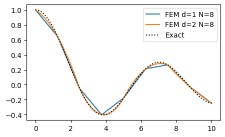
Since we now know how to assemble any matrix, we can also solve any (linear) ordinary differential equation. Let us try to solve Poisson’s equation with a manufactured solution \(u(x) = J_0(x), \, x \in [0, 10]\), where \(J_0(x)\) is the 0 order Bessel function of the first kind. We first create a function fem_poisson that solves the problem using any order \(d\) and any right hand side function \(f(x)\).

from fem import assemble_b, fe_evaluate_v

def fem_poisson(N, f, d=1, domain=(0, 1), bc=(0, 0)):
    xj = np.linspace(domain[0], domain[1], N+1)
    S = -assemble_generic_matrix(xj, d, 1, 1)
    S[0, 1:] = 0; S[0, 0] = 1    # ident first row for bc at u(0)
    S[-1, 1:] = 0; S[-1, -1] = 1 # ident last row for bc at u(L)
    b = assemble_b(f, xj, d=d)
    b[0] = bc[0]   # specify u(0)
    b[-1] = bc[1]  # specify u(L)
    uh = np.linalg.solve(S, b)
    return uh

We can now solve the problem using any order. But remember, the number of nodes need to match the order of the method. A method of order \(d\) need to use \(N=d M\) for some integer \(M\).

ue = sp.besselj(0, x)
f = ue.diff(x, 2)
bc = (ue.subs(x, 0), ue.subs(x, 10))

fig = plt.figure(figsize=(5, 3))
ax = fig.gca()
for d in (1, 2):
    N = 8
    uh = fem_poisson(N, f, d=d, domain=(0, 10), bc=bc)
    mesh = np.linspace(0, 10, N+1)
    xj = np.linspace(0, 10, 100)
    ax.plot(xj, fe_evaluate_v(uh, xj, mesh, d=d))
ax.plot(xj, sp.lambdify(x, ue)(xj), 'k:')
ax.legend([f'FEM d=1 N={N}', f'FEM d=2 N={N}', 'Exact']);

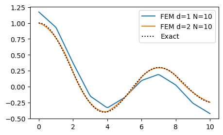
Neumann boundary conditions

We will now solve a Helmholtz equation with Neumann boundary conditions

(59)\[ u'' + \alpha u= f, \quad x \in (0, L), \, u'(0) = a, u'(L) = b. \]

Note

If \(\alpha=0\), then Eq. (59) becomes Poisson’s equation. In this case the problem is ill-defined and we need to add another constraint, like in lecture 11. The Helmholtz problem is well-defined and does not require a constraint.

The Neumann problem is solved with the same Lagrange polynomials and space \(V_N\) as the Dirichlet problem. With the Galerkin method we get the variational form

(60)\[ -(u_N', v') + \alpha(u_N, v) = (f, v) - [u_N'v]_{x=0}^{x=L}, \quad \forall \, v \in V_N. \]

Here we already know how to assemble \((u_N', v'), (u_N, v)\) and \((f, v)\). The only new issue is boundary conditions. We no longer know \(\hat{u}_0\) or \(\hat{u}_N\), but we do know that \(u'(0)=a\) and \(u'(L)=b\). If we first insert for \(u_N\) and \(v = \psi_i\) and manipulate just a little bit we get

(61)\[ \sum_{j=0}^N \left(-(\psi'_j, \psi'_i) +\alpha(\psi_j, \psi_i)\right) \hat{u}_j = (f, \psi_i) - \left(u'_N(L)\psi_i(L) - u'_N(0)\psi_i(0)\right). \]

The two boundary conditions can be inserted into the two boundary terms above and we get

(62)\[ \sum_{j=0}^N \left(-(\psi'_j, \psi'_i) +\alpha(\psi_j, \psi_i)\right) \hat{u}_j = (f, \psi_i) - b\psi_i(L) + a\psi_i(0), \]

which is the Helmholtz equation to solve with Neumann boundary conditions. Note that the boundary conditions will enter the equations for \(\hat{u}_0\) and \(\hat{u}_N\), because \(\psi_i(0)\) and \(\psi_i(L)\) are only nonzero for \(i=0\) and \(i=N\), respectively. In fact, \(\psi_0(0)=1\) and \(\psi_N(L)=1\).

We solve Eq. (62) as a linear algebra problem

\[ (-S+\alpha A) \boldsymbol{\hat{u}} = \boldsymbol{b}, \]

where \(s_{ij} = (\psi'_j, \psi'_i), a_{ij}=(\psi_j, \psi_i)\) and the right hand side vector \(\boldsymbol{b}\) becomes

\[\begin{split} \boldsymbol{b} = \begin{bmatrix} (f, \psi_0)+a \\ (f, \psi_1) \\ \vdots \\ (f, \psi_{N-1}) \\ (f, \psi_N) - b \end{bmatrix} \end{split}\]

def fem_poisson_neumann(N, f, alpha=1, d=1, domain=(0, 1), bc=(0, 0)):
    xj = np.linspace(domain[0], domain[1], N+1)
    S = -assemble_generic_matrix(xj, d, 1, 1)
    A = assemble_generic_matrix(xj, d, 0, 0)
    b = assemble_b(f, xj, d=d)
    b[0] += bc[0]   # specify u'(0)
    b[-1] -= bc[1]  # specify u'(L)
    uh = np.linalg.solve(S+alpha*A, b)
    return uh

ue = sp.besselj(0, x)
alpha = 0.1
f = ue.diff(x, 2)+alpha*ue
bc = (ue.diff(x, 1).subs(x, 0).n(), ue.diff(x, 1).subs(x, 10).n())

fig = plt.figure(figsize=(5, 3))
ax = fig.gca()
for d in (1, 2):
    N = 10
    uh = fem_poisson_neumann(N, f, alpha, d=d, domain=(0, 10), bc=bc)
    mesh = np.linspace(0, 10, N+1)
    xj = np.linspace(0, 10, 100)
    ax.plot(xj, fe_evaluate_v(uh, xj, mesh, d=d))
ax.plot(xj, sp.lambdify(x, ue)(xj), 'k:')
ax.legend([f'FEM d=1 N={N}', f'FEM d=2 N={N}', 'Exact']);

Note

None of the matrices \(S\) or \(A\) are affected in any way by the Neumann boundary conditions. The Neumann condition only applies to the right hand side vector \(\boldsymbol{b}\).

FEM in multiple dimensions

The finite element method is particularly useful in 2D or 3D because the method can handle geometrically complex domains \(\Omega\) with ease. The method is still exactly as in 1D, but now the basis functions are multidimensional

\[ u(x, y, z) \approx u_N(x, y, z) = \sum_{j=0}^N \hat{u}_j \psi_j(x, y, z). \]

The function space is also the same \(V_N = \text{span}\{\psi_j\}_{j=0}^N\) and we still solve for \(u_N \in V_N\) such that

\[ (\mathcal{L}(u_N)-f, v)_{L^2(\Omega)} = 0, \quad \forall \, v \in V_N, \]

for some \(\mathcal{L}(u_N)\). So it is still only a matter of choosing basis functions, and then the rest follows more or less mechanically. However, in 2D and 3D we deal with partial differential equations (PDEs) and normally describe the equations using the gradient and divergence operators. Poisson’s equation is normally written as

\[ \nabla^2 u = f, \]

where \(\nabla^2 u = \nabla \cdot \nabla u = \text{div}(\text{grad}(u))\). On variational form Poisson’s equation becomes

\[ (\nabla^2 u, v)_{L^2(\Omega)} = (f, v)_{L^2(\Omega)}. \]

The \(L^2(\Omega)\) inner product is defined for multiple dimensions as

\[ (u, v)_{L^2(\Omega)} = \int_{\Omega}u \cdot v \, d\Omega, \]

where \(u\) and \(v\) can be either scalar or vector fields, which is why we need the dot product on the right hand side in the integral.

In multiple dimensions we cannot use integration by parts, which is defined only for one dimension, but the exact same idea extends to multiple dimensions using Green’s first identity

Green’s first identity

Green’s first identity can be written as

\[ \int_{\Omega} \nabla^2 u \,v \,d\Omega = -\int_{\Omega} \nabla u \cdot \nabla v \, d \Omega + \oint_{\partial \Omega} \nabla u \cdot \boldsymbol{n} \, v \, d \sigma, \]

where \(\partial \Omega\) is the enclosing boundary of the domain \(\Omega\), \(\boldsymbol{n}\) is an outward pointing unit normal vector and \(d\sigma\) is a line element in 2D and a surface element in 3D. We can also write Green’s identity using the \(L^2\) inner product notation

\[ (\nabla^2 u, v)_{L^2(\Omega)} = - (\nabla u, \nabla v)_{L^2(\Omega)} + (\nabla u \cdot \boldsymbol{n}, v)_{L^2(\partial \Omega)}. \]

Note the use of \(L^2(\partial \Omega)\) for the line- or surface-integral.

Note

Sometimes you see the following notation for the gradient of \(u\) in the direction normal to \(\partial \Omega\):

\[ \frac{\partial u}{\partial n} = \nabla u \cdot \boldsymbol{n} \]

By applying Green’s first identity to the Poisson problem we get

\[ -(\nabla u, \nabla v)_{L^2(\Omega)} = (f, v)_{L^2(\Omega)} - (\nabla u \cdot \boldsymbol{n}, v)_{L^2(\partial \Omega)}. \]

Exactly like in 1D Neumann boundary conditions are fixed though the boundary term \((\nabla u \cdot \boldsymbol{n}, v)_{L^2(\partial \Omega)}\), whereas Dirichlet conditions are specified by fixing \(\hat{u}_i\) for all points \(i\) where the mesh point \(\boldsymbol{x}_i=(x_i, y_i, z_i)\) is on the boundary. As in 1D Dirichlet boundary conditions are implemented by identing all rows in the coefficient matrix corresponding to a boundary point and manipulating the right hand side vector.

A problem is often declared with Neumann on some part of the domain and Dirichlet on another. We then normally declare the problem as

\[ \mathcal{L}(u) = f, \quad \boldsymbol{x} \in \Omega, \quad u(\boldsymbol{x}) = u_0, \boldsymbol{x} \in \partial \Omega_D, \quad \frac{\partial u}{\partial n}(\boldsymbol{x}) = g, \boldsymbol{x} \in \partial \Omega_N. \]

where \(\partial \Omega_D\) and \(\partial \Omega_N\) are the parts of the boundary where Dirichlet and Neumann boundary conditions should be applied, respectively.

A major difference from global Galerkin methods is that it is not common to use tensor products for multiple dimensions. Instead we use multidimensional basis functions \(\psi_j(x,y,z)\) and just the single sum

\[ u_N(\boldsymbol{x}) = \sum_{j=0}^N \hat{u}_j \psi_j(\boldsymbol{x}). \]

On the contrary, with tensor product methods there is one basis function for each dimension and we use approximations like

\[ u_N(x, y) = \sum_{i=0}^M\sum_{j=0}^N \hat{u}_{ij}\psi_{i}(x) \varphi_j(y), \]

in 2D and three sums over three basis functions in 3D.

The multidimensional basis functions are usually defined on reference elements. Remember that we earlier in 1D mapped all elements to a reference domain \(X \in [-1, 1]\). In 2D and 3D we use instead reference triangles and tetrahedra as shown in Fig. 6

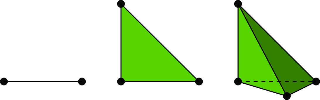
Fig. 6 P1 finite element reference elements in 1D, 2D and 3D. The dots are the nodes in the elements.

The piecewise linear basis function \(\psi_j(\boldsymbol{x})\) now live on a 2D mesh consisting of triangles, but \(\psi_j(\boldsymbol{x}_i)\) is still 1 if \(i=j\) and 0 otherwise. In other words the piecewise linear basis functions are still defined such that

\[ \psi_j(\boldsymbol{x}_i) = \delta_{ij}, \]

for all nodes \(\boldsymbol{x}_i\) in the computational mesh. This leads to the “tent” basis function that is nicely illustrated in Fig. 7

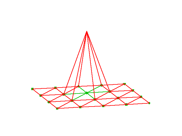
Fig. 7 Illustration of one single basis function \(\psi_j(\boldsymbol{x})\), where the node in the center of the “tent” is \(\boldsymbol{x}_j\) such that \(\psi_j(\boldsymbol{x}_j)=1\) at this node only and zero on all the others.

The reference triangle has three nodes \(\boldsymbol{X}_0= (0, 0), \boldsymbol{X}_1= (1, 0)\) and \( \boldsymbol{X}_2 = (0, 1)\), and the three nonzero reference basis functions on this element are

\[ \tilde{\psi}_0(X, Y) = 1-X-Y, \quad \tilde{\psi}_1(X, Y) = X, \quad \tilde{\psi}_2(X, Y) = Y. \]

This should be compared with the Lagrange polynomials on the 1D reference element (41). Note that the reference basis functions are mapped as

\[ \psi_{q(e, r)}(\boldsymbol{x}) = \tilde{\psi}_r(\boldsymbol{X}). \]

There is a mapping \(q(e, r)\) from local to global degrees of freedom also in multiple dimensions, but the mapping is not as easy as (39). Normally, the finite element in multiple dimensions is implemented in an unstructured manner, and the map from a local node \(r\) on a global element \(e\), \(q(e, r)\), needs to be stored in lists.

Note

We write boldface \(\boldsymbol{x}\) for a point in physical space and \(\boldsymbol{X}\) for a point in reference space. For a global node \(i = q(e,r)\) on local node \(r\) on element \(e\), the node is \(\boldsymbol{x}_i = \boldsymbol{x}_{q(e, r)}\). For local node \(r\) the reference point is \(\boldsymbol{X}_r\). In 2D and 3D \(\boldsymbol{x}_i\) is respectively \((x_i, y_i)\) and \((x_i, y_i, z_i)\) and \(\boldsymbol{X}_r\) is \((X_r, Y_r)\) and \((X_r, Y_r, Z_r)\). We will also use \(\boldsymbol{x} = (x_0, x_1, x_2)\) and \(\boldsymbol{X} = (X_0, X_1, X_2)\) if we need to loop over coordinates.

We can map from the reference coordinate \(\boldsymbol{X}\) to the physical coordinate \(\boldsymbol{x}\) using

(63)\[ \boldsymbol{x} = \sum_{r} \tilde{\psi}_r(\boldsymbol{X}) \boldsymbol{x}_{q(e, r)}, \]

where \(r\) runs over the number of vertices on the reference element, i.e., 2 on lines, 3 on triangles and 4 on tetrahedra. You should try to convince yourself that (63) is the same as Eq. (40) on a line.

Assembly of element matrices in 2D or 3D

Lets consider the assembly of the element stiffness matrix

(64)\[ \int_{\Omega^{(e)}} \nabla \psi_j(\boldsymbol{x}) \cdot \nabla \psi_i(\boldsymbol{x}) \, d\Omega, \]

where \(\psi_j(\boldsymbol{x})\) is the basis function \(j\) defined in physical space. Suppose that we now want to compute this integral using the reference elements \(\tilde{\Omega}^{(r)}\) and the reference basis functions \(\tilde{\psi}_r(\boldsymbol{X}) = \psi_{q(e, r)}(\boldsymbol{x}) = \psi_j(\boldsymbol{x})\).

A change of variables in the integral leads to a change in domain from \(\Omega^{(e)}\) to \(\tilde{\Omega}^{(r)}\), and the volume element changes into

\[ d\Omega = \text{det}J \, d\tilde{\Omega}, \]

where \(J\) is the Jacobian matrix of the transformation from \(\boldsymbol{x}\) to \(\boldsymbol{X}\). The Jacobian and its inverse are defined as

\[ J_{i,j} = \frac{\partial x_j}{\partial X_i} \quad \text{and} \quad J^{-1}_{i,j} = \frac{\partial X_j}{\partial x_i}. \]

We also need to transform the derivatives present in the integral (64). The \(i\)’th component of the gradient in physical space can be written as

\[ (\nabla \psi_j)_i = \frac{\partial \psi_j}{ \partial x_i}, \]

and we can transform these derivatives as

\[ \frac{\partial \psi_{q(e, r)}(\boldsymbol{x})}{\partial x_i} =\frac{\partial \tilde{\psi}_r(\boldsymbol{X})}{\partial x_i} = \frac{\partial \tilde{\psi}_r}{\partial X_j}\frac{\partial X_j}{\partial x_i}, \]

with summation implied by repeating indices. Using the inverse Jacobian we can write the last term as

(65)\[ \frac{\partial \tilde{\psi}_r}{\partial X_j}\frac{\partial X_j}{\partial x_i} = J_{ij}^{-1} \frac{\partial \tilde{\psi}_r}{\partial X_j}. \]

We can also define this on matrix form using

\[\begin{split} \nabla u= \begin{bmatrix} \frac{\partial u}{\partial x} \\[0.1cm] \frac{\partial u}{\partial y} \\[0.1cm] \frac{\partial u}{\partial z} \end{bmatrix} \quad \text{and} \quad \nabla_X u = \begin{bmatrix} \frac{\partial u}{\partial X} \\[0.1cm] \frac{\partial u}{\partial Y} \\[0.1cm] \frac{\partial u}{\partial Z} \end{bmatrix}. \end{split}\]

We then get (65) as

\[ \nabla \psi_{q(e, r)} = J^{-1} \cdot \nabla_X \tilde{\psi}_r \]

Inserted into (64) we get

\[ \int_{\Omega^{(e)}} \nabla \psi_{q(e, s)}(\boldsymbol{x}) \cdot \nabla \psi_{q(e, r)}(\boldsymbol{x}) \, d\Omega = \int_{\tilde{\Omega}^{(r)}} \left(J^{-1} \cdot \nabla_X \tilde{\psi}_s(\boldsymbol{X})\right) \cdot \left(J^{-1} \cdot \nabla_X \tilde{\psi}_r(\boldsymbol{X})\right) \, \text{det}J\, d\tilde{\Omega}. \]

Quite complicated, but like for 1D you can compute the reference integral once and then reuse it for all future purposes.

Implementing the finite element in two or three dimensions on unstructured grids is a bit too complex for this short course. But there are excellent software tools available for free that can help you implement very complex equations in even more complex domains. See, e.g.,

• FEniCS

• Elmer

• FreeFEM

• and more

FEniCS is very nice since it has an easy to use Python interface, and it has been developed partly at UiO.