Lecture 13 - Time-dependent variational methods#
In lecture 11 and lecture 12 we have focused on the spatial discretization of steady (time-independent) differential equations. We will now add time-dependence and thus consider equations like
The solution \(u(\boldsymbol{x}, t)\) is now a function of both space \(\boldsymbol{x}\) and time \(t\), and naturally, the approximation will be as well. However, we will put all the time dependence in the expansion coefficients
and the spatial dependence in the basis functions. As such, we still use the same (time-independent) function space \(V_N = \text{span}\{\psi_j\}_{j=0}^N\), and the above sum is equivalent to the expansion \(u_N(\boldsymbol{x}, t) \in V_N\).
The most common approach for handling time-dependent problems with variational methods is to use a finite difference method for the time-derivative, and then subsequently apply the method of weighted residuals. For example, in order to solve
with the forward Euler method in time, we discretize first as
where \(u^n(\boldsymbol{x}) = u(\boldsymbol{x}, t_n)\), \(f^n(\boldsymbol{x}) = f(\boldsymbol{x}, t_n)\) and \(t_n=n \Delta t\).
Note
For simplicity we normally drop the spatial dependence and write only \(u^n\) and \(f^n\), even though we mean \(u^n(\boldsymbol{x})\) and \(f^n(\boldsymbol{x})\).
The solution \(u^n\) is known and \(u^{n+1}\) is the unknown we are after. As always the Euler method needs to initialize the solution \(u^0\) in order to get started.
A residual can now be defined as
and as always we want this residual to be zero.
Note
The notation \(\mathcal{R}(u^{n+1}; u^n)\) is used to indicate that \(u^{n+1}\) is the unknown and \(u^n\) (right of the semicolon) is known.
We now introduce the approximations to \(u^{k}(\boldsymbol{x}) = u(\boldsymbol{x}, t_k)\), which for given integer \(k\) is found in the space \(V_N\)
Inserted into the residual we get
The method of weighted residuals is to find \(u^{n+1}_N \in V_N\) such that
and for the Galerkin method \(W = V_N\).
In order to solve the time-dependent problem we need to solve this Galerkin problem many times. The procedure is
Initialize \(u_N^0(\boldsymbol{x})\)
For \(n = 0, 1, \ldots, N_t-1\) find \(u^{n+1}_N \in V_N\) such that
Here \(N_t\) is the number of time steps such that \(N_t \Delta t = T\) and \(t \in (0, T]\).
Note
By initializing \(u_N^0(\boldsymbol{x})=u^0(\boldsymbol{x})\), we need to project \(u^0(\boldsymbol{x})\) to \(V_N\) and store the expansion coefficients \(\boldsymbol{\hat{u}}^0\). This is a regular function approximation, like in lectures 8 and 9. For the finite difference method, on the other hand, initialization is simply to evaluate (interpolate) the solution on the computational mesh: \((u^0(x_i))_{i=0}^N\). The finite element method can do either project or interpolate, because the FEM is using Lagrange polynomials such that \(u_N(x_i) = \hat{u}_i\).
Stability#
Just like for the finite difference method we need to be very careful with the time step \(\Delta t\), in order to obtain a stable solution. A stable solution is one that remains bounded as \(t \longrightarrow \infty\). However, there is one major difference from the finite difference or collocation methods. The Galerkin method described above does not involve a mesh size \(\Delta x\)! So the Courant number is not defined. How do we overcome this problem? In order to describe this problem it is helpful to first revisit the stability of the finite difference method.
Stability of the forward Euler method for finite difference spatial discretizations#
We start by considering (67) with finite difference discretizations for both temporal and spatial derivatives:
where, for example, \(\mathcal{L}(\boldsymbol{u}^n)_j = (u^n_{j+1}-2u^n_j+u^n_{j-1})/\Delta x^2\) if \(\mathcal{L}\) represents the second derivative \(\partial^2/\partial x^2\). For simplicity we have assumed only one spatial dimension and the mesh function is thus \(u^n_j=u(x_j, t_n)\), where \(x_j = j \Delta x\) and \(t_n = n \Delta t\). The solution vector at a given time step \(n\) is given as \(\boldsymbol{u}^n = (u^n_j)_{j=0}^N\).
With the finite difference method we assume that the solution can be written as an exponential decay in time and periodic in space (the Fourier wave \(e^{ikx_j}\) is periodic in space)
where \(i = \sqrt{-1}\) and \(k\) is a wavenumber. The spatial mesh is \( \boldsymbol{x} = (x_j)_{j=0}^N\) and we will write this ansatz as
where \(g=e^{a \Delta t}\) is the amplification factor, which is independent of space and time, and only depends on \(\Delta t\) and \(\Delta x\). We now let the operator \(\mathcal{L}\) be the finite difference \(m\)’th derivative operator \(D^{(m)}=(d^{(m)}_{ij})_{i,j=0}^N\), such that
For example, if \(m=2\) and we use second order accuracy, then \(\sum_{k}d_{jk}^{(2)}{u}_k^n = (u^n_{j+1}-2u^n_j+u^n_{j-1})/\Delta x^2\). With matrix notation we can write
Now apply the ansatz \(\boldsymbol{u}^n=g^n \boldsymbol{u}^0\), such that
Divide by \(g^n\) to obtain
Stability requires that \(|g| \le 1\). However, unlike the decay equation discussed in lectures 1 and 2, it is not always a requirement that \(g>0\), because the solution may be oscillatory.
In order to say something more specific about stability, we need to define the finite difference matrix \(D^{(m)}\). So lets assume for now that \(m=2\) and use the derivative matrix with periodic boundary conditions
where \(h=\Delta x\) and \(D^{(2)} = {h^{-2}} \tilde{D}^{(2)}\), where \(\tilde{D}^{(2)}\) is the matrix in (69) without the \(h^{-2}\) scaling. We get
and inserting for \({u}_j^0=e^{ik j \Delta x}\) we get
Divide by \(e^{ikj\Delta x}\) to obtain
and use \(e^{ix}+e^{-ix} = 2 \cos x\), \(\cos(2x) = \cos^2 x - \sin^2 x\) and \(1=\cos^2x+\sin^2x\) to obtain
We still want \(|g|\le 1\), so we need
and since \(\sin^2\left(k \Delta x/2\right) \le 1\) and positive, we get that \(1- \frac{4 \Delta t}{\Delta x^2}\) is always less than 1. However, \(1- \frac{4 \Delta t}{\Delta x^2}\) can be smaller than \(-1\), and that gives us the limit
which is satisfied if \(\Delta t/\Delta x^2 \le 1/2\). This is the absolute stability limit for the forward Euler method for the diffusion equation. Note that it involves both \(\Delta t\) and \(\Delta x\).
We have now found the absolute stability limit for the diffusion equation using the forward Euler method. However, it was quite complicated to compute since we had to discretize in both space and time. You might ask if there is an easier way, and the answer for once is yes. There is actually a generic approach we can take for any differentiation matrix (any value of \(m\) in \(D^{(m)}\)), and that is to compute its eigenvalues \(\lambda\), such that
We can insert this into (68) to obtain
which indicates that \(g-1 = \Delta t \lambda\). So we can compute the amplification factor \(g\) from the eigenvalues of the difference matrix! Since we require that \(|g| \le 1\), we get that
which is a generic result for the forward Euler method with any difference matrix \(D^{(m)}\). Note that \(\lambda\) are the eigenvalues of \(D^{(m)}\), which is a matrix that includes \(\Delta x\). In the case of \(D^{(2)}\), we could also find the eigenvalues of \(\tilde{D}^{(2)}\), which would be the same as for \(D^{(2)}\), but divided by \(\Delta x^2\). With \(\lambda\) the eigenvalues of \(\tilde{D}^{(2)}\), we get the more specific result for the diffusion equation
We can now compute the eigenvalues of \(\tilde{D}^{(2)}\)
import numpy as np
from scipy import sparse

N = 11
D2 = sparse.diags((1, 1, -2, 1, 1), (-N, -1, 0, 1, N), shape=(N+1, N+1))
Lambda = np.linalg.eig(D2.toarray())[0]
print(f"Minimum eigenvalue = {min(Lambda)}")
Minimum eigenvalue = -3.9999999999999973
We find that the minimum eigenvalue is -4! And we get the same result using any odd \(N\). Hence we get
which is the same result as (70) if we set \(\sin^2(k \Delta x/2)\) to its maximum value of 1.
Stability of the forward Euler method for variational forms#
As described in the start of Stability, the variational methods do not include a mesh size \(\Delta x\). However, we can use the eigenvalue approach described above without defining a mesh size and we will now use this to find stability limits for variational forms.
First of all we make the same ansatz and assume that the solution \(u_N^{n+1}\) can be computed from \(u_N^n\) as
where \(g\) is an amplification factor independent of spatial coordinate \(x\). As always a stable method is one where \(|g| < 1\).
For the forward Euler method we now consider the discretized Galerkin equation
and insert for Eq. (72)
Divide by \(g^n\) (\(g\) is not dependent on \(x\)) to obtain
We now insert for \(u^0_N = \sum_{j=0}^N \hat{u}^0_j \psi_j\) and \(v=\psi_i\) to obtain
On matrix form this is
where \(A\) is the mass matrix and \(m_{ij} = \left( \mathcal{L}(\psi_j), \psi_i\right)\) and \(M=(m_{ij})_{i,j=0}^N\). Multiply from the left by \(A^{-1}\) to obtain
We can compute the eigenvalues \(\lambda\) of the matrix \(H = A^{-1}M\) such that
which can be inserted into (74)
Since the vector \(\boldsymbol{\hat{u}}^0\) is the same in all three terms, we get that
and for stability \(|g| \le 1\), we need to have \(|1+\lambda \Delta t| \le 1\).
So with the Galerkin method we do not need the mesh size \(\Delta x\) in order to compute stability limits. On the other hand, we do need to solve an eigenvalue problem to find the eigenvalues \(\lambda\). In the stability computation, we use the largest eigenvalue. Lets try this out with a complete example, using the diffusion equation.
The diffusion equation#
Consider the diffusion equation with Dirichlet boundary conditions and a prescribed initial condition
In order to solve (75) we choose a global Galerkin method with mapped Legendre polynomials and basis functions \(\psi_i(x)=P_i(X)-P_{i+2}(X)\) such that \(V_N = \text{span}\{\psi_i\}_{i=0}^N\). We then use Eq. (73) and create a linear algebra problem by inserting for \(u^{n+1}_N, u^n_N\) and \(v=\psi_i\) and using integrating by parts on the diffusion term:
Since we are using basis functions that are all zero on the boundaries, the last term disappears. In order to incorporate the Dirichlet boundary condition we add a boundary term \(B(x)\) and solve for \(\tilde{u}^{n+1}_N = u^{n+1}_N - B(x)\), where \(\tilde{u}^{n+1}_N(0, t) = \tilde{u}^{n+1}_N(L, t)=0\). Note that we get exactly the same equation for \(u^{n+1}_N\) as for \(\tilde{u}^{n+1}_N\) since all terms with \(B(x)\) will be eliminated when inserting \(u^{n+1}_N = \tilde{u}^{n+1}_N+B(x)\) and \(u^{n}_N = \tilde{u}^{n}_N+B(x)\). But we solve the equation for \(\tilde{u}^{n+1}_N\), with the zero boundary conditions, and then to get \(u^{n+1}_N\) we simply add \(B(x)\).
We use Legendre basis functions with a mapping from \(x\in[0, L]\) to \(X \in [-1, 1]\) such that
The stiffness matrix \(s_{ij} = (\psi'_j, \psi'_i)\) was given in Eq. (51), but it needs to be modified for the mapping
The mass matrix \(a_{ij} = (\psi_j, \psi_i)\) is similarly
The mass matrix is symmetric and we know that \((P_j, P_i) = \|P_i\|^2 \delta_{ij}\), where \(\|P_i\|^2=\frac{2}{2i+1}\) is the squared \(L^2\) norm of \(P_i\). Hence with \(j = i\) we get
and with \(j=i+2\) we get
The mass matrix is as such
On matrix form the equation to solve is
This equation is solved for \(n = 0, 1, \ldots, N_t-1\), after first initializing \(\boldsymbol{\hat{u}}^0\).
A solver is created in the class FE_Diffusion below, where we reuse the code from mandatory assignment 2. In the code we assemble the mass and stiffness matrices \(A\) and \(S\), and compute the eigenvalues \(\lambda\) of \(H=A^{-1}S\). We then use that \(|1-\lambda \Delta t| \le 1\) (where the minus is because we have used integration by parts) and the fact that here all eigenvalues are positive real numbers, to determine that
This means that for stability we need to choose a time step \(\Delta t \le 2/\max(\lambda)\).
import numpy as np
import sympy as sp
from scipy import sparse
from galerkin import TrialFunction, TestFunction, DirichletLegendre, DirichletChebyshev, \
    project, inner

x, t, c, L = sp.symbols('x,t,c,L')

class FE_Diffusion:
    """Class for solving the diffusion equation with

    Parameters
    ----------
    N : int
        Number of basis functions
    L0 : number
        The extent of the domain, which is [0, L0]
    bc : 2-tuple of numbers
        The Dirichlet boundary conditions at the two edges
    u0 : Sympy function of x, t, c and L
        Used for specifying initial condition
    """
    def __init__(self, N, L0=1, u0=sp.cos(sp.pi*x/L)+sp.cos(10*sp.pi*x/L)):
        self.N = N
        self.L = L0
        self.u0 = u0.subs({L: L0})
        self.bc = (self.u0.subs({x: 0, t: 0}).n(), self.u0.subs({x: L0, t: 0}).n())
        self.uh_np1 = np.zeros(N+1) # expansion coefficients \hat{u}^{n+1}
        self.uh_n = np.zeros(N+1)
        self.V = self.get_function_space()
        self.A, self.S = self.get_mats()
        self.lu = sparse.linalg.splu(self.A.tocsc())

    def get_function_space(self):
        return DirichletLegendre(self.N, domain=(0, self.L), bc=self.bc)

    def get_mats(self):
        """Return mass and stiffness matrices
        """
        N = self.N
        u = TrialFunction(self.V)
        v = TestFunction(self.V)
        a = inner(u, v)
        s = 2/self.L*sparse.diags([4*np.arange(N+1)+6], [0], shape=(N+1, N+1), format='csr')
        return a, s

    def get_eigenvalues(self):
        """Return eigenvalues of H=A^{-1}S"""
        return np.linalg.eig(np.linalg.inv(self.A.toarray()) @ self.S.toarray())[0]

    def __call__(self, Nt, dt=0.1, save_step=100):
        """Solve diffusion equation

        Parameters
        ----------
        Nt : int
            Number of time steps
        dt : number
            timestep
        save_step : int, optional
            Save solution every save_step time step

        Returns
        -------
        Dictionary with key, values as timestep, array of solution
        The number of items in the dictionary is Nt/save_step, and
        each value is an array of length N+1

        """
        # Initialize
        self.uh_n[:] = project(self.u0, self.V) # unm1 = u(x, 0)
        xj = self.V.mesh()
        plotdata = {0: self.V.eval(self.uh_n, xj)}

        # Solve
        f = np.zeros(self.N+1)
        for n in range(2, Nt+1):
            f[:] = self.A @ self.uh_n - dt*(self.S @ self.uh_n)
            self.uh_np1[:] = self.lu.solve(f)
            self.uh_n[:] = self.uh_np1
            if n % save_step == 0: # save every save_step timestep
                plotdata[n] = self.V.eval(self.uh_np1, xj)
        return plotdata
Lets solve the problem using initial condition \(u(x, 0) = \cos(\pi x /L) + \cos(10 \pi x/L)\) and \(dt= 2/\max(\lambda)\):
from utilities import plot_with_offset
sol = FE_Diffusion(40, L0=2)
dt = 2/max(sol.get_eigenvalues())
data = sol(1000, dt=dt, save_step=100)
plot_with_offset(data, sol.V.mesh(), figsize=(4, 3))
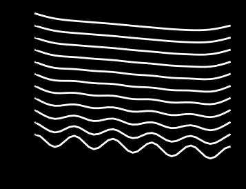
The solution is nice and smooth and the time step is
print(f'Maximum time step = {dt}')
Maximum time step = 2.198057879034515e-05
Lets solve it using a slightly larger \(dt\) to see if this really is the largest possible time step:
data = sol(1000, dt=1.01*dt, save_step=100)
plot_with_offset(data, sol.V.mesh(), figsize=(4, 3))
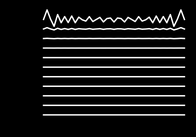
Obviously, the solver is now unstable and the solution diverges.
Note
The diffusion equation is “stiff” and requires a very short time step with the forward Euler method in order to remain stable.
Changing from Legendre to Chebyshev makes the required time step even shorter.
class FE_Diffusion_Cheb(FE_Diffusion):

    def get_function_space(self):
        return DirichletChebyshev(self.N, domain=(0, self.L), bc=self.bc)

    def get_mats(self):
        """Return mass and stiffness matrices
        """
        N = self.N
        u = TrialFunction(self.V)
        v = TestFunction(self.V)
        a = inner(u, v)
        #s2 = -inner(u.diff(2), v) # slow
        k = np.arange(N+1, dtype=float)
        def diag(i):
            if i == 0:
                return 2*np.pi*(k+1)*(k+2)
            return 4*np.pi*(k[:-(i)]+1)
        diags = np.arange(0, N+1, 2)
        vals = [diag(i) for i in diags]
        s = 2/self.L * sparse.diags(vals, diags, shape=(N+1, N+1), format='csr')
        return a, s
sol = FE_Diffusion_Cheb(40, L0=2)
dt = 2/max(sol.get_eigenvalues())
data = sol(1000, dt=dt, save_step=100)
plot_with_offset(data, sol.V.mesh(), figsize=(4, 3))
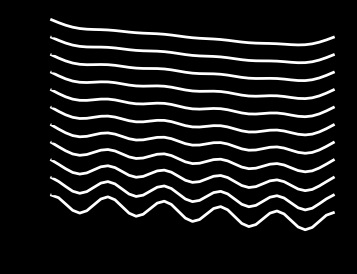
print(f'Maximum time step = {dt}')
Maximum time step = 1.233224916131476e-05
We can compare the absolute stability limits with the finite difference method, where \(\Delta t/\Delta x^2 \le 0.5\) for stability. Using a uniform mesh with \(N=40\), we get \(\Delta x = 2/N = 0.05\) and \(\Delta t \le 0.5 \cdot 0.05^2 = 1.25 \cdot 10^{-3}\). Hence, the Galerkin method with Chebyshev basis functions requires approximately 100 times shorter time steps for stability!
Stiffness matrix for Chebyshev basis
Note that in the implementation we have used \(s_{ij} = -(\psi''_j, \psi_i)_{\omega}\) and
because it is quite expensive to compute the matrix using the inner(u.diff(2), v) function that loops over all \(i,j \in \mathcal{I}_N^2\). Equation (76) can be derived using
but it is a lot of work and only necessary in order to save some time on computing the stiffness matrix.
Also note that because of the non-constant weight function \(\omega(x)=1/\sqrt{1-x^2}\) it is not common to use integration by parts with the Chebyshev basis.
Use a stencil matrix for the implementation#
It is rather messy to work with composite basis functions. A very smart trick is thus to use a stencil matrix \(S\), such that (summation on repeated \(j\) index)
This defines \(S \in \mathbb{R}^{(N+1) \times (N+3)}\) for the Dirichlet problem as
With \(\boldsymbol{\psi} = \{\psi_i\}_{i=0}^N\) and \(\boldsymbol{P}=\{P_i\}_{i=0}^{N+2}\) (note the longer vector) we get all basis functions in matrix form:
But why is the stencil matrix so smart? Consider the mass matrix
You need to sort out the four (diagonal) matrices on the right. This is not very difficult, since they are all diagonal, but you need to watch out for the indices in order for the mass matrix to turn out correctly. Now use stencil matrix instead (with summation on \(k\) and \(l\)):
Here you only need the one diagonal matrix \(P = ((P_l, P_k))_{k,l=0}^{N+2,N+2}\), where \((P_l, P_k)=\frac{2}{2l+1}\delta_{kl}\). The great advantage only becomes apparent in matrix form though
And this works for any stencil matrix, not just the Dirichlet one. That is the main advantage of the stencil matrix approach. For the Neumann basis (see lecture 11)
the stencil matrix is
where \(\alpha = N(N+1)/((N+2)(N+3))\). The stiffness matrix can also be computed through the stencil matrix:
Again you need only the single matrix using orthogonal polynomials \(q_{kl}=(P''_l, P_k) = -(P'_l, P'_k)\) and the matrix form is again much simpler:
Backward Euler#
The forward Euler method requires a very short time step for the diffusion equation. How about the backward Euler method
where the only difference from forward is that \(\left(\mathcal{L}(u^{n+1}_N), v\right)\) is making use of the unknown \(u^{n+1}_N\) and not the known \(u^n_N\)? The linear algebra problem is now
If we continue with the ansatz \(u^{n+1}_N = g u^n_N\), and thus \(u^{n+1}_N = g^{n+1} u^0_N\), we get
which on matrix form reads
If we multiply from left to right by \(A^{-1}\) we get
Here we can once again use \(H=A^{-1}S\) and \(H \boldsymbol{\hat{u}}^0 = \lambda \boldsymbol{\hat{u}}^0\) and thus we find
Since all time steps and eigenvalues are real numbers larger than 0, we find that \(g\) is always less than 1 and the backward Euler method is as such unconditionally stable.
The Wave equation#
Lets consider the wave equation from lecture 5 in one spatial dimension
As you may recall, we solved the wave equation with Dirichlet, Neumann and open boundary conditions. The two time derivatives also required that the solution was initialized at two time-steps, or more mathematically precise, that both \(u({x}, 0)\) and \(\frac{\partial u}{\partial t}({x}, 0)\) were given.
We now use finite differences in time such that
A numerical residual \(\mathcal{R}_N = \mathcal{R}(u^{n+1}_N; u^n_N, u^{n-1}_N)\) can now be defined as
where we use \(\alpha = c \Delta t\) and \(u' = \frac{\partial u}{\partial x}\) for simplicity, since there is only one spatial dimension. If we now initialize \(u_N^0\) and \(u_N^1\), the Galerkin method is to find \(u^{n+1}_N \in V_N\) such that
for \(n = 1, \ldots, N_t-1\). We can also integrate the last term by parts
In order to solve the Galerkin problem we need to formulate the linear algebra problem. Hence we insert for \(u^{n-1}_N, u^{n}_N, u^{n+1}_N\) and \(v = \psi_i\) to obtain
We next rearrange such that the unknown \(\hat{u}_j^{n+1}\) is on the left hand side and the rest of the known terms are on the right hand side
With matrix notation, \(a_{ij} = (\psi_j, \psi_i)\) and \(s_{ij} = (\psi'_j, \psi'_i) \), we get
where \(\boldsymbol{b}^n = ((u^n_N)'(L) \psi_i(L) - (u^n_N)'(0) \psi_i(0))_{i=0}^N\). We can write this as
where the vector \(\boldsymbol{f}^n = A (2 \boldsymbol{\hat{u}}^n - \boldsymbol{\hat{u}}^{n-1}) - \alpha^2 \left( S \boldsymbol{\hat{u}}^n - \boldsymbol{b}^n\right) \).
The boundary conditions determine the path forward. Here there are subtile differences between global Galerkin methods and the local finite element method, but the procedures are exactly as detailed in lecture 11 and lecture 12.
For Dirichlet boundary conditions \(u(0, t) = a\) and \(u(L, t) = b\):
Global methods make use of basis functions that are all zero at the boundaries \(\psi_j(0) =\psi_j(L) = 0\). Hence the vector \(\boldsymbol{b}^n\) disappears. Nonzero values for \(a, b\) are incorporated using a boundary function, see lecture 11.
The finite element method makes use of Lagrange polynomials and \(\psi_i(0)= 1\) for \(i=0\) and zero otherwise. Similarly, \(\psi_i(L)=1 \) for \(i=N\) and zero otherwise. Hence it is only \(b^n_0\) and \(b^n_N\) that potentially are different from zero. However, since \(u(0, t)=a = \hat{u}^{n+1}_0\) and \(u(L, t) = b = \hat{u}^{n+1}_N\) we ident \(A\) and set \(f^n_0=a\) and \(f^n_N=b\) (see lecture 12). As such the boundary terms in \(\boldsymbol{b}^n\) will never enter the equation system.
For Neumann boundary conditions \(u'(0, t) = g_0\) and \(u'(L, t) = g_L\):
Global methods can make use of basis functions that all have \(\psi'_j(0) = \psi'_j(L)=0\), and add a boundary function \(B(x)\) that satisfied \(B'(0)=g_0\) and \(B'(L)=g_L\). However, global methods can also make use of any basis functions (like pure Legendre polynomials) and incorporate the boundary conditions through \(\boldsymbol{b}^n\). We get that \(b^n_i = g_L\psi_i(L)-g_0\psi_i(0)\). Note that this approach is very easy to use if \(g_0=g_L=0\), because in that case you only need to neglect the boundary vector \(\boldsymbol{b}^n\).
The finite element method makes use of the weak form and specifies \(b^n_0 = -g_0\) and \(b^n_N = g_L\) since the basis functions are Lagrange polynomials. No more is needed. In the event that \(g_0 = g_L = 0\), the boundary vector can simply be neglected.
How about stability? We can make the same ansatz as for the diffusion equation and assume \(u_N^{n+1}=g^{n+1}u_N^0\). We get after some trivial manipulations
which can be transformed by dividing by \(g^n\) and multiplying by \(A^{-1}\) from the left
Using \(H = A^{-1} S\) and \(H \boldsymbol{\hat{u}}^0 = \lambda \boldsymbol{\hat{u}}^0\), we get
where \( \beta = -\alpha^2 \lambda +2\). This is more difficult to conclude with than for the Euler method, because we have a quadratic equation for \(g\). Nevertheless, we can find
and in order for \(|g| \le 1\) (\(g\) may be complex) we need \(-2 \le \beta \le 2\) and thus \(0 \le \alpha^2 \lambda \le 4\). The maximum time step that we can use is as such
Note
For all \(-2 \le \beta \le 2\) we get that \(|g|=1\). This makes sense if we consider \(g + g^{-1} = \beta\), because if \(g\) is a root of the quadratic equation, then \(g^{-1}\) must also be a root. Hence, if \(g < 1\), then \(g^{-1}>1\), which is unstable. So all the possible \(\beta\) must here have \(|g|=1\). We can also easily compute \(|\beta \pm \sqrt{\beta^2-4}| = 2\) when the real number \(-2 \le \beta \le 2\).
Lets implement the wave equation using a global Galerkin method, homogeneous Dirichlet boundary conditions and an initial pulse \(u(x, t) = \exp(-200(x-L/2+ct)^2)\) used for both \(t=0\) and \(t=\Delta t\). Since we are using the same matrices as the diffusion problem, we can create a solver by subclassing the FE_Diffusion class and thus reuse much code
class Wave(FE_Diffusion):
    def __init__(self, N, L0=1, c0=1, u0=sp.cos(sp.pi*x/L)+sp.cos(10*sp.pi*x/L)):
        u0 = u0.subs({c: c0})
        FE_Diffusion.__init__(self, N, L0=L0, u0=u0)
        self.c = c0
        self.uh_nm1 = np.zeros_like(self.uh_n)

    def __call__(self, Nt, dt=0.1, save_step=100):
        # Initialize
        self.uh_nm1[:] = project(self.u0.subs(t, 0), self.V) # unm1 = u(x, 0)
        xj = self.V.mesh()
        plotdata = {0: self.V.eval(self.uh_nm1, xj)}
        self.uh_n[:] = project(self.u0.subs(t, dt), self.V)
        if save_step == 1:
            plotdata[1] = self.V.eval(self.uh_n, xj)

        # Solve
        f = np.zeros(self.N+1)
        alfa = self.c*dt
        for n in range(2, Nt+1):
            f[:] = self.A @ (2*self.uh_n-self.uh_nm1) - alfa**2*(self.S @ self.uh_n)
            self.uh_np1[:] = self.lu.solve(f)
            self.uh_nm1[:] = self.uh_n
            self.uh_n[:] = self.uh_np1
            if n % save_step == 0: # save every save_step timestep
                plotdata[n] = self.V.eval(self.uh_np1, xj)
        return plotdata
sol = Wave(40, L0=2, c0=1, u0=sp.exp(-50*(x-L/2+c*t)**2))
dt = 1/sol.c*np.sqrt(4/max(sol.get_eigenvalues()))
data = sol(400, dt=dt, save_step=40)
plot_with_offset(data, sol.V.mesh(), figsize=(4, 3))
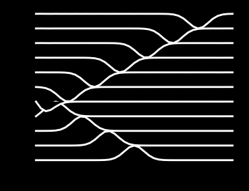
print(f"Maximum time step = {dt}")
Maximum time step = 0.006630321076742083
This maximum time step should be compared with the maximum time step of a finite difference method. Remember the Courant number \(C = c \Delta t/\Delta x\) and the stability condition \(C \le 1\). For our case, with \(c=1\), this limit is \(\Delta t \le \Delta x\). So with \(N=40\) and \(\Delta x = 2/N\), we get \(\Delta t \le 0.05\). Again, the finite difference method can take much longer time steps than the global Galerkin method. But remember, the global Galerkin method is using a much more accurate spatial discretization and can actually get away with using a much lower \(N\).
Weekly assignments#
Implement the diffusion equation with the backward Euler scheme.
Find the absolute stability limit of the diffusion equation discretized with a Crank-Nicolson scheme. Use both a finite difference method \( \boldsymbol{u}^{n+1} - \boldsymbol{u}^n = \frac{\Delta t}{2}D^{(2)}(\boldsymbol{u}^{n+1}+\boldsymbol{u}^n) \) and a comparable Galerkin method.
Implement the diffusion equation with a Crank-Nicolson scheme and verify the absolute stability limits found in 2.
Consider the leap-frog finite difference scheme \( \boldsymbol{u}^{n+1} - \boldsymbol{u}^{n-1} = {2\Delta t}D^{(2)}\boldsymbol{u}^n, \) suggested by Richardson in 1910. Explain why this scheme is unconditionally unstable. To this end you can use that all the eigenvalues of \(D^{(2)}\) are real.
Note
Richardson was one of the great pioneers for using mathematical techniques in weather forecasting, but at the time (1910) he did not know about stability limits for finite difference schemes. The von Neumann stability analysis that made this possible was not discovered until 1947.