Lecture 7 - Postprocessing and interpolation#
In lecture 7 we will be mostly concerned with postprocessing, which is the analysis of the solution after it has been computed. Important topics are
One and two-dimensional interpolation
Lagrange interpolation polynomials
Interpolation of derivatives
Integration over boundaries
The wave equation in 2D
Postprocessing and Interpolation#
We have up until now focussed solely on how to solve equations using finite difference stencils and mesh functions evaluated on a regular (uniform) mesh. For example, in 1D a mesh function is
where \(x_i = i \Delta x\). In 2D a mesh function is
where \(y_j = j \Delta y\). We have also looked at a problem that is 1D in space, plus time. In this case the mesh function is
where \(t_n = n \Delta t\). Later in this lecture we will look at the wave equation in 2D space plus time. In this case the mesh function will be
Up until now we have learned how to compute these mesh functions, but we have not really talked about how to use them. In a real project we are often interested in specific measures, like drag or flowrate, that can be measured at a single point, line or at a surface. In that case you may need to find the solution or its derivative at specific points that are not mesh points. How do you compute this number from the mesh function? And how do you integrate over a line or a surface?
The answer to the first question is interpolation. The second will require a numerical integration scheme.
One-dimensional interpolation#
Interpolation is easily illustrated through a one-dimensional example. Assume that the mesh domain is \(\Omega \in [0, 1]\) and
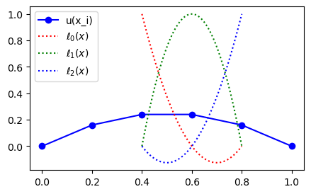
Create a uniform mesh \(\boldsymbol{x}=(i/N)_{i=0}^N\) using \(N=5\) and plot the mesh function corresponding to (8) as blue dots.
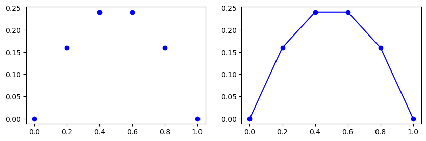
In the figure above to the left the mesh function \(U=(u_i)_{i=0}^N\) is represented with the blue dots. In the figure to the right linear profiles have been added by matplotlib in between the points because we ask for it using bo-. The linear profiles represent linear interpolation, which is a first order approach to computing the mesh function in between the mesh points. The next figure compares the linear interpolation to the exact solution.
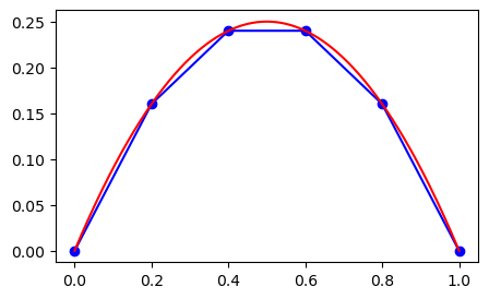
Note that even though the mesh function here is exact at all the mesh points, the linear interpolation between points is far from being accurate.
We now want to compute \(u(0.75)\) using linear interpolation. We get this from drawing a straight line from \(u(x_3=0.6) = 0.24\) to \(u(x_4=0.8)=0.16\), and this line can be represented as
By inserting for \(u_3, u_4, x_3\) and \(x_4\) we get
We can create this profile using Sympy
x = sp.Symbol('x')
uo = u[3] + (u[4]-u[3])/(xj[4]-xj[3])*(x-xj[3])
uo
And we can plot the linearly interpolated point \(u(0.75)\) as a green dot
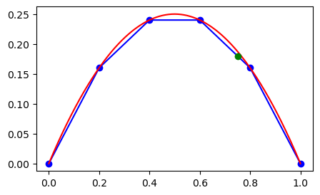
The interpolation curve that we have created using Sympy can be used for any point, but it makes most sense to use it between \(x_3\) and \(x_4\). If we use it outside this domain, the accuracy is much worse, and we also refer to this as extrapolation.
Lagrange interpolation polynomials#
Linear interpolation is easy to understand and easy to compute with. However, it is not very accurate. And why would you want to waste your hard earned second-order accurate mesh function (or exact, as above) using only first order accurate interpolation? You shouldn’t and there is no need to. Linear interpolation makes use of only 2 interpolation points. Higher order interpolation simply makes use of more points. The most straight-forward way to do this is through the use of Lagrange interpolation polynomials.
A Lagrange interpolation polynomial makes use of a set of \(k+1\) nodes \(\{x^0, x^1, \ldots, x^k\}\). These are not usually identical to the entire computational mesh, but rather the closest points to the point of interest. Like for the linear interpolation above, the points would simply be \(\{x^0, x^1\} = \{x_3, x_4\}\) for linear interpolation, or \(\{x^0, x^1, x^2\} = \{x_2, x_3, x_4\}\) for second order.
Note
To separate the Lagrange points from the mesh points we will simply use superscript on the Lagrange points. So here the superscript does not mean the power!
With Lagrange interpolation we make use of the Lagrange basis functions (or cardinal functions)
which can be more compactly written as
The Lagrange basis functions can be easily implemented using Sympy:
def Lagrangebasis(xj, x=x):
"""Construct Lagrange basis for points in xj
Parameters
----------
xj : array
Interpolation points (nodes)
x : Sympy Symbol
Returns
-------
Lagrange basis as a list of Sympy functions
"""
from sympy import Mul
n = len(xj)
ell = []
numert = Mul(*[x - xj[i] for i in range(n)])
for i in range(n):
numer = numert/(x - xj[i])
denom = Mul(*[(xj[i] - xj[j]) for j in range(n) if i != j])
ell.append(numer/denom)
return ell
We can plot some of the basis functions, for example for second order interpolation using \(\{x^0, x^1, x^2\} = \{x_2, x_3, x_4\}\)
ell = Lagrangebasis(xj[2:5], x=x)
for l in ell:
print(l)
12.5*(x - 0.8)*(x - 0.6)
-25.0*(x - 0.8)*(x - 0.4)
12.5*(x - 0.6)*(x - 0.4)
Note
Note that all Lagrange basis functions are such that on the chosen mesh points \(\{x^{i}\}_{i=0}^{k}\) we have
Note
The Lagrange basis functions do not depend on the mesh function values, only on the mesh points. Also note that the mesh points do not need to be uniform, any mesh will do as long as all points are different.
The Lagrange interpolating polynomial is defined as
where \(u^j\) are the mesh function values at the chosen mesh points \(x^j\). Note that for the linear interpolation example, we would use the two neighbouring values \(\{u^0, u^1\} = \{u_3, u_4\}\).
Because of (9) we automatically get that
since
and \(\ell_j(x^i) = 1\) for \(i=j\), whereas \(\ell_j(x^i) = 0\) for all \(i \ne j\).
The Python function Lagrangefunction returns the complete Lagrange function:
def Lagrangefunction(u, basis):
"""Return Lagrange polynomial
Parameters
----------
u : array
Mesh function values
basis : tuple of Lagrange basis functions
Output from Lagrangebasis
"""
f = 0
for j, uj in enumerate(u):
f += basis[j]*uj
return f
Let us try this new function and see if we can reproduce the linear interpolation function that we have already computed above:
ell = Lagrangebasis(xj[3:5])
L = Lagrangefunction(u[3:5], ell)
print(L)
0.48 - 0.4*x
Works!
Term by term this is
The Lagrange polynomial is then
Inserting for \(u^0=0.24, u^1=0.16, x^0=0.6\) and \(x^1=0.8\) we get
which can be rearranged into
which is the same as the linear interpolation we have already computed before.
Note
Higher order interpolation simply makes use of more neighbouring points.
ell = Lagrangebasis(xj[2:6])
L = Lagrangefunction(u[2:6], ell)
L
We can evaluate the Lagrange polynomial for an array of points as well:
sp.lambdify(x, L)(np.array([0.5, 0.6, 0.7]))
array([0.25, 0.24, 0.21])
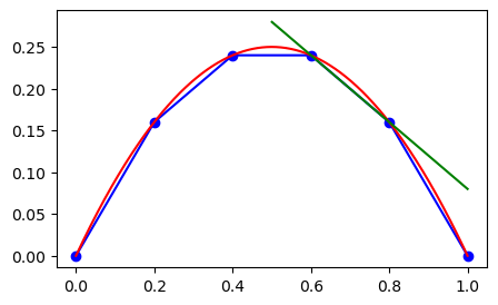
Interpolation of derivatives#
Lagrange polynomials can be used to evaluate \(u(x)\) inside a domain when the mesh function \(u(x_i)\) is known. But how can we evaluate derivatives \(u'(x)\)? The most natural approach is perhaps to use a finite difference stencil that computes the derivative at all mesh points
With the matrix \(D^{(1)}\)
import scipy.sparse as sparse
D1 = sparse.diags([-1, 1], [-1, 1], (N+1, N+1), 'lil')
D1[0, :3] = -3, 4, -1
D1[-1, -3:] = 1, -4, 3
D1 *= (N/2)
du = D1 @ u
du
array([ 1. , 0.6, 0.2, -0.2, -0.6, -1. ])
With the derivative available at all mesh points, we can do interpolation with Lagrange interpolation polynomials, exactly like before, only using the mesh function \(u'(x_j)\) instead of \(u(x_j)\).
Lp = Lagrangefunction(du[2:6], ell)
print(Lp.subs(x, 0.75))
-0.500000000000000
This result is exact since \(u(x) = x(1-x)\) and thus \(u'(x)=1-2x\) leading to \(u'(0.75)=1-2\cdot 0.75 = -0.5\).
However, this is a rather costly operation since it involves a matrix and the solution at all mesh points. Is it possible to do better?
Well, we already have the mesh function \(u(x_j)\) and the Lagrange polynomial
This polynomial is an ordinary function and as such it can be differentiated
We can thus use the Lagrange polynomial that we have created between mesh points \(\{x_2, x_3, x_4, x_5\}\), which is currently stored in L:
dL = sp.diff(L, x)
print(dL.subs(x, 0.75))
-0.500000000000000
This works exactly because we have chosen a second order polynomial as mesh function and the derivative is a linear polynomial \(1-2x\). But the approach is generic and we do not have to compute \(u'(x)\) on the entire mesh, we can simply use the mesh function (that is already computed) and the Lagrange polynomials.
Two-dimensional interpolation#
We now consider the 2D problem where we have the mesh function
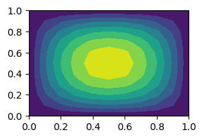
and want to evaluate this mesh function for some point inside the domain that is not a mesh point. We now need to interpolate in two dimensions. To get started we need a 2D mesh and an appropriate mesh function to interpolate. We will use the 2D function
and a domain \(\Omega = [0, 1]^2\).
Note
It is common to write \([a, b]^2\) for the Cartesian product of a set with itself. So \([0, 1]^2 = [0, 1] \times [0, 1]\)
def mesh2D(Nx, Ny, Lx, Ly, sparse=False):
x = np.linspace(0, Lx, Nx+1)
y = np.linspace(0, Ly, Ny+1)
return np.meshgrid(x, y, indexing='ij', sparse=sparse)
N = 10
xij, yij = mesh2D(N, N, 1, 1, False)
u2 = xij*(1-xij)*yij*(1-yij)
plt.figure(figsize=(3, 2))
plt.contourf(xij, yij, u2);
We want to find \(u(0.55, 0.65)\) from the mesh function \(U=(u_{ij})_{i,j=0}^{N, N}\).
There are several procedures for performing 2D interpolation. We will choose the Lagrange interpolation first and use \(k+1\) points in both \(x\) and \(y\) directions. In this case the Lagrange interpolating polynomial will be
where \(u^{m,n}\) are the mesh function values for the points we choose for the interpolation, that should be the points closest to the interpolated point. For our case with \(N=10\) this would be the four points \((u_{ij})_{i=5, j=6}^{6, 7}\).
The four interpolation points are shown as blue dots in the figure below, and the point we are trying to evaluate is shown as a red dot

The Lagrange basis functions \(\ell_m(x)\) and \(\ell_n(y)\) are computed exactly as before, only now with \(\ell_m(x)\) using points along the \(x\)-direction (for linear \(\{x^0, x^1\}=\{x_5, x_6\})\) whereas \(\ell_n(y)\) are using points along the \(y\)-direction (for linear \(\{y^0, y^1\}=\{y_6, y_7\}\)). Naturally, we can choose more points if we want more than linear interpolation.
We can reuse the previously defined function Lagrangebasis, since both \(\ell_m(x)\) and \(\ell_n(y)\) are one-dimensional functions. This was the reason why we gave Lagrangebasis a keyword argument x=x, because now we can compute \(\ell_n(y)\) using a Symbol y as shown below:
y = sp.Symbol('y')
lx = Lagrangebasis(xij[5:7, 0], x=x)
ly = Lagrangebasis(yij[0, 6:8], x=y)
We need a new function for the 2D Lagrange polynomial though, since this is a double loop
def Lagrangefunction2D(u, basisx, basisy):
N, M = u.shape
f = 0
for i in range(N):
for j in range(M):
f += basisx[i]*basisy[j]*u[i, j]
return f
Lagrangefunction2D should return a Lagrange function like (10).
We can now test the function by first creating it
f = Lagrangefunction2D(u2[5:7, 6:8], lx, ly)
f
sp.simplify(f)
and then checking that it works
ue = x*(1-x)*y*(1-y)
print(f.subs({x: 0.55, y: 0.65}), ue.subs({x: 0.55, y: 0.65}))
0.0551250000000000 0.0563062500000000
The results are not identical because this is merely a first order interpolation. With one additional point using \((x_5, x_6, x_7)\) and \((y_5, y_6, y_7)\) we get
lx = Lagrangebasis(xij[5:8, 0], x=x)
ly = Lagrangebasis(yij[0, 5:8], x=y)
L2 = Lagrangefunction2D(u2[5:8, 5:8], lx, ly)
print(L2.subs({x: 0.55, y: 0.65}), ue.subs({x: 0.55, y: 0.65}))
0.0563062500000000 0.0563062500000000
These two results are now identical since the polynomials are second order.
Partial derivatives#
We can compute partial derivatives in 2D, much like we did for the 1D case. We compute the derivatives from the mesh function \(U = (u_{ij})_{i,j=0}^{N_x, N_y}\) as
The results will both be new mesh functions defined on the entire mesh. Like in 1D this is unnecessary if all you want is to compute only the derivative in a single point. In that case you can, again like in 1D, take the derivative of the Lagrange polynomial
Try this with Sympy and verify with analytical solution:
dLx = sp.diff(L2, x)
dLy = sp.diff(L2, y)
print(dLx.subs({x: 0.55, y: 0.65}), sp.diff(ue, x).subs({x: 0.55, y: 0.65}))
-0.0227500000000000 -0.0227500000000000
Other tools for interpolation#
There are also other tools in Numpy and Scipy that can help you do 2D interpolation with minimal effort. Most of them are based on splines, which is not a topic in this class, but still useful to know about. We can do interpolation with simple, one-line calls, as follows
from scipy.interpolate import interpn
print(interpn((xij[5:8, 0], yij[0, 5:8]), u2[5:8, 5:8], np.array([0.55, 0.65])))
[0.055125]
Here we get the same result as linear above even though we use 3 points in each direction. This is because interpn is using linear interpolation by default. Modify this to cubic (which requires 4 points in each direction) to obtain better accuracy
print(interpn((xij[5:9, 0], yij[0, 5:9]), u2[5:9, 5:9], np.array([0.55, 0.65]), method='cubic'))
[0.05630625]
Errors and integration#
For the numerical solution \(u\) and the exact solution \(u^{e}\) the \(L^2\) error norm can in general, for any domain \(\Omega\) and number of dimensions, be defined as
In 2D \(\Omega = [0, L_x] \times [0, L_y]\) and the integral becomes
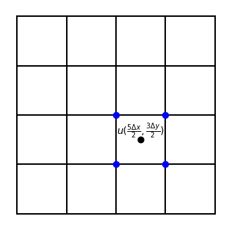
Hence we need to be able to compute such double integrals. One approach is the midpoint rule computed for any integrand \(u(x, y)\) as follows
This integral requires the value of the function \(u\) in the middle of all the computational cells, where the cells are defined as all the squares in the figure below. In order to compute the value of \(u\) in the center of all cells, we need to interpolate. Linear interpolation will in this case lead to an average of \(u\) in the four surrounding nodes, marked with blue dots in the figure for \(u(2.5 \Delta x, 1.5 \Delta y)\).
Lets create a mesh function from an analytical solution
N = 20
xij, yij = mesh2D(N, N, 1, 1, False)
u2 = np.cos(xij)*(1-xij)*np.sin(yij)*(1-yij)
ue = sp.cos(x)*(1-x)*sp.sin(y)*(1-y)
We can compute values of \(u\) in all the cell centers easily using vectorization. For the field u2 defined above with shape \((N_x+1)\times (N_y+1)\) we get
um = (u2[:-1, :-1]+u2[1:, :-1]+u2[:-1, 1:]+u2[1:, 1:])/4
Note that um is a matrix of shape \(N_x \times N_y\).
The integral required for the \(L^2\)-norm can now be computed easily and we get the following function for the \(L^2\) error
def L2_error(u, dx, dy):
um = (u[:-1, :-1]+u[1:, :-1]+u[:-1, 1:]+u[1:, 1:])/4
return np.sqrt(np.sum(um**2*dx*dy))
ua = sp.lambdify((x, y), ue)(xij, yij)
L2_error(u2-ua, 1/N, 1/N)
np.float64(5.108490959653866e-18)
The result is close to machine precision, which it should be because the Lagrange interpolator produces results identical to the mesh function at all mesh points. Hence, to test the integral, we can send in just the mesh function instead:
L2_error(u2, 1/N, 1/N)
np.float64(0.09552823074589575)
The exact answer is close
float(sp.sqrt(sp.integrate(sp.integrate(ue**2, (y, 0, 1)), (x, 0, 1))))
0.09586332023451888
Just like for the 1D case there is a simplification using the small \(\ell^2\) norm instead
The result will be very similar to the \(L^2\)-norm for most mesh functions. Note how the sums are from 0 to \(N_x\) and \(N_y\) above, since these are sums over nodes and not cell centers. The \(l^2\) error is very easy to implement:
def l2_error(u, dx, dy):
return np.sqrt(dx*dy*np.sum(u**2))
l2_error(u2, 1/N, 1/N)
np.float64(0.09980275105614006)
which is less accurate than the midpoint rule, but still useful as an error measure. (Note that this \(\ell^2\) norm is not really supposed to represent the integral exactly, and as such it makes little sense to compare the number to the integral.)
You can also use nested trapz or Simpson’s rule for the integration:
def L2_error_trapz(u, dx, dy):
return np.sqrt(np.trapz(np.trapz(u**2, dx=dy, axis=1), dx=dx))
L2_error_trapz(u2, 1/N, 1/N)
/var/folders/ql/nly59sfj4dd3spkth6lk0kjw0000gn/T/ipykernel_55605/4021080097.py:2: DeprecationWarning: `trapz` is deprecated. Use `trapezoid` instead, or one of the numerical integration functions in `scipy.integrate`.
return np.sqrt(np.trapz(np.trapz(u**2, dx=dy, axis=1), dx=dx))
np.float64(0.09592899344305951)
def L2_error_simps(u, dx, dy):
from scipy.integrate import simpson as simp
return np.sqrt(simp(simp(u**2, dx=dy, axis=1), dx=dx))
L2_error_simps(u2, 1/N, 1/N)
np.float64(0.09586418448463656)
Integration over boundary#
In many real problems we are interested in average values, or values integrated over a boundary. For example, to compute lift and drag on an airfoil wing you need to integrate both pressure and friction forces over the entire wing boundary. We do not yet have such complicated geometries here, but it is still useful to know how to compute integrals over boundaries. Like for the \(L^2\) error norm we will need to use numerical integration.
Let us compute the measure \(\overline{u}(y) = \int_{0}^{L_x} u(x, y) dx\). Note that the result is a function of \(y\), but not \(x\) since we integrate over the \(x\)-direction.
def integrate_x(u, dx):
return np.trapz(u, dx=dx, axis=0)
integrate_x(u2, 1/N)
/var/folders/ql/nly59sfj4dd3spkth6lk0kjw0000gn/T/ipykernel_55605/1693027423.py:2: DeprecationWarning: `trapz` is deprecated. Use `trapezoid` instead, or one of the numerical integration functions in `scipy.integrate`.
return np.trapz(u, dx=dx, axis=0)
array([0. , 0.02183109, 0.04131248, 0.05840408, 0.07307749,
0.08531604, 0.09511478, 0.10248041, 0.10743121, 0.10999687,
0.11021837, 0.10814768, 0.10384757, 0.09739127, 0.08886213,
0.07835326, 0.06596713, 0.05181507, 0.03601686, 0.01870016,
0. ])
The result is an array of numbers, one for each column index in the matrix u2. The result is a function of \(y\). If we only want to compute the integral on one of the two boundaries with constant \(y\), then it is less expensive to choose the \(j\) index before integrating. This can be done as follows:
def integrate_boundary_x(u, dx, j=0):
return np.trapz(u[:, j], dx=dx, axis=0)
integrate_boundary_x(u2, 1/N, j=0)
/var/folders/ql/nly59sfj4dd3spkth6lk0kjw0000gn/T/ipykernel_55605/345090187.py:2: DeprecationWarning: `trapz` is deprecated. Use `trapezoid` instead, or one of the numerical integration functions in `scipy.integrate`.
return np.trapz(u[:, j], dx=dx, axis=0)
np.float64(0.0)
Computing drag requires the integral of derivatives, like \(\int_{0}^{L_x} \frac{\partial u(x, y)}{\partial y} dx\). For the boundary located at \(y=0\) we would then need the mesh function \(\frac{\partial u}{\partial y} (x_i, y_0)\) before integrating. Here we can use only the first row of the derivative matrix in \(U(D^{(1)})^T\), which simplifies to the following forward difference
Having computed \(\frac{\partial u(x_i, y_0)}{\partial y}\) we can simply use the trapezoidal integration on the resulting array.
duy = (N/2)*(-3*u2[:, 0] + 4*u2[:, 1] - u2[:, 2])
np.trapz(duy, dx=1/N)
/var/folders/ql/nly59sfj4dd3spkth6lk0kjw0000gn/T/ipykernel_55605/1824253925.py:2: DeprecationWarning: `trapz` is deprecated. Use `trapezoid` instead, or one of the numerical integration functions in `scipy.integrate`.
np.trapz(duy, dx=1/N)
np.float64(0.46011886423778525)
Let us verify the result using Sympy
dudye = sp.diff(ue, y)
sp.integrate(dudye.subs(y, 0), (x, 0, 1)).n()
This seems to be correct, but it should be further verified using refinement of the mesh.
The wave equation in 2D plus time#
We will now consider the wave equation
in a two-dimensional spatial domain \(\Omega = [0, L_x] \times [0, L_y]\) and in time \(t \in [0, T]\). The problem will be solved with Dirichlet boundary conditions \(u=0\) on the entire boundary, and it will also require an initial condition \(u(0, x, y) = I(x, y)\) and an initial derivative, here set to zero \(\frac{\partial u}{\partial t}(0, x, y) = 0\).
Perhaps surprisingly, this equation is considerably easier to implement than the Poisson equation, because of the hyperbolic nature of the problem. Hyperbolic problems are often solved with marching methods that simply step the solution forward in time, and do as such not require setting up and solving matrix equations. However, we can still use much of the theory described in lecture 6, about the 2D mesh and 2D discretised equations.
Note
Time-dependent equations like the wave-equation (hyperbolic) are usually easy to implement, but the numerical scheme needs to consider stability as the solution is moved forward in time. Steady-state equations like the Poisson equation (elliptic) are usually more difficult to set up, but stability is then usually not an issue because we are not stepping the solution anywhere (unless we try to solve the problem iteratively).
Mesh function#
The computational mesh is the same as in lecture 6, with the domain
and mesh \(\boldsymbol{x} \times \boldsymbol{y}\) where
and \(\Delta x = L_x/N_x\) and \(\Delta y = L_y/N_y\).
Time will also use uniform intervals, and \(t_n = n \Delta t\) for \(n=0, 1, \ldots, N_t\). A function \(u(t, x, y)\) evaluated on this mesh is now found as
However, we will only store the solution at three consecutive time steps, just like for the 1D wave problem. We will as such make use of the three mesh functions
that all are matrices of shape \((N_x+1) \times (N_y+1)\).
We will solve the wave equation using central difference in time as well as in space. A discretization of all internal points is thus
In matrix form this equation reads
The initial condition \(\frac{\partial u}{\partial t}(0, x, y) = 0\) can be implemented like we did in lecture 5 for the wave equation with one spatial dimension. We use
in the PDE for \(n=0\)
such that
A solution algorithm is thus to
Specify \(U^0\) and \(U^1\) from initial conditions
for n in (1, 2, …, \(N_t-1\)) compute
\(U^{n+1} = 2U^n - U^{n-1} + (c\Delta t)^2 \left( D^{(2)}_x U^n + U^n (D^{(2)}_y)^T \right)\)
Apply boundary conditions to \(U^{n+1}\)
Swap \(U^{n-1} \leftarrow U^n\) and \(U^n \leftarrow U^{n+1}\)
Other than that we can simply reuse a lot of code from lecture 6. A function for the second derivative matrix is:
import numpy as np
import scipy.sparse as sparse
def D2(N):
D = sparse.diags([1, -2, 1], [-1, 0, 1], (N+1, N+1), 'lil')
D[0, :4] = 2, -5, 4, -1
D[-1, -4:] = -1, 4, -5, 2
return D
A function mesh2D for creating the 2D mesh has already been described in this notebook. We are thus ready to create a solver that steps the solution forward in time. For simplicity we will use \(N_x=N_y=N\) and \(L_x=L_y=L\)
def solver(N, L, Nt, cfl=0.5, c=1, store_data=10,
u0=lambda x, y: np.exp(-40*((x-0.6)**2+(y-0.5)**2))):
xij, yij = mesh2D(N, N, L, L)
Unp1, Un, Unm1 = np.zeros((3, N+1, N+1))
Unm1[:] = u0(xij, yij)
dx = L / N
D = D2(N)/dx**2
dt = cfl*dx/c
Un[:] = Unm1[:] + 0.5*(c*dt)**2*(D @ Unm1 + Unm1 @ D.T)
plotdata = {0: Unm1.copy()}
if store_data == 1:
plotdata[1] = Un.copy()
for n in range(1, Nt):
Unp1[:] = 2*Un - Unm1 + (c*dt)**2*(D @ Un + Un @ D.T)
# Set boundary conditions
Unp1[0] = 0
Unp1[-1] = 0
Unp1[:, -1] = 0
Unp1[:, 0] = 0
# Swap solutions
Unm1[:] = Un
Un[:] = Unp1
if n % store_data == 0:
plotdata[n] = Unm1.copy() # Unm1 is now swapped to Un
return xij, yij, plotdata
Note that boundary conditions can be set after stepping the solution forward in time. Hence it does not really matter what is done to the solution at boundaries when Unp1 is computed, because the boundary will be modified later. This is very different from when we solve the Poisson equation and it is possible because of the recursive (explicit) solution algorithm. Note that the unknown Unp1 is not part of the right hand side in the update
A vectorized algorithm for this problem is possible, and it would read
However, this approach is not necessary, since we use a recursive solution algorithm that simply updates \(U^{n+1}\). Note that if we were to write this vectorized equation as Ax=b, then A would simply be equal to the identity matrix and b would be equal to the entire right hand side above. Since A is the identity matrix, the linear algebra problem is already taken care of. For the Poisson equation it is different because A equals \(D^{(2)}_x \otimes I_y + I_x \otimes D^{(2)}_y\). As stated initially, the hyperbolic nature of the wave equation makes it significantly easier to solve than the elliptic Poisson equation.
We are now ready to solve the wave equation for a chosen mesh size and we also choose to store the solution every fifth time step.
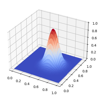
xij, yij, data = solver(40, 1, 171, cfl=0.71, store_data=5)
Plot the initial data
from matplotlib import cm
fig, ax = plt.subplots(subplot_kw={"projection": "3d"})
surf = ax.plot_surface(xij, yij, data[0], cmap=cm.coolwarm,
linewidth=0, antialiased=False)
Create an animation for the solution using matplotlib.
%%capture
# capture, otherwise there will be a plot in this cell
import matplotlib.animation as animation
fig, ax = plt.subplots(subplot_kw={"projection": "3d"})
frames = []
for n, val in data.items():
frame = ax.plot_wireframe(xij, yij, val, rstride=2, cstride=2);
#frame = ax.plot_surface(xij, yij, val, vmin=-0.5*data[0].max(),
# vmax=data[0].max(), cmap=cm.coolwarm,
# linewidth=0, antialiased=False)
frames.append([frame])
ani = animation.ArtistAnimation(fig, frames, interval=400, blit=True,
repeat_delay=1000)
ani.save('wavemovie2dunstable.apng', writer='pillow', fps=5) # This animated png opens in a browser
from IPython.display import HTML
from IPython.display import display
display(HTML(ani.to_jshtml()))
Note that the CFL number \(C = c \Delta t / \Delta x\) here needs to be smaller than \(1/\sqrt{2}\) in order to get a stable solution. This number follows from the two-dimensional nature of the problem where the wave can spread out in two dimensions. Try to solve the problem above with CFL=1 and it should blow up.
Note that there is usually one CFL number for each direction in a two-dimensional problem:
and for the current problem you need (see Eq. (2.97) in the PDE book)
which for \(\Delta x = \Delta y\) leads to \(\frac{c \Delta t}{ \Delta x} \le \frac{1}{\sqrt{2}}\).