Lecture 4

Initial Value Problems (IVPs)

Up until now we have considered the exponential decay model and the vibration equation. We have studied the problems as recurrence relations, or marching problems. Such problems specify initial conditions at the outset of the simulation, and then moves the solution forward in time from that point. Such problems are also classified as Initial Value Problems (IVPs).

The marching methods are very easy to implement intuitively using for-loops. The solution at \(u^{n+1}\) is simply computed from the previous solutions \(u^n, u^{n-1}, \ldots\) and there is really no need for linear algebra.

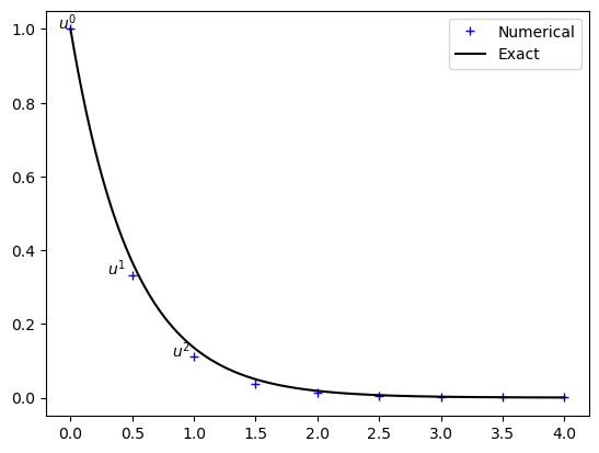
We have previously considered the decay model

\[ u' + au = 0, t \in (0, T], \, u(0)=I. \]

In order to solve this problem we create a solution vector \(\boldsymbol{u} = (u^0, u^1, \ldots, u^{N_t})\), set \(u^0=I\) and continue to solve the recurrence relation

\[ \frac{u^{n+1}-u^n}{\Delta t} = -a (\theta u^{n+1} + (1-\theta) u^n) \quad \text{for}\, n=1, 2, \ldots, N.\]

Rearranged

\[ u^{n+1} = \frac{1 - (1-\theta) a \Delta t}{1 + \theta a \Delta t} u^n = g u^n \]

where \(g = \frac{1 - (1-\theta) a \Delta t}{1 + \theta a \Delta t}\) is the amplification factor.

Recurrence algorithm:

• \(u^0 = I\)

• for n = 0, 1, … , N-1

  • Compute \(u^{n+1} = g u^n\)

import numpy as np
import matplotlib.pyplot as plt
np.set_printoptions(precision=3, suppress=True)
N = 8
a = 2
I = 1
theta = 0.5
dt = 0.5
T = N*dt
t = np.linspace(0, N*dt, N+1)
u = np.zeros(N+1)
g = (1 - (1-theta) * a * dt)/(1 + theta * a * dt)
u[0] = I
for n in range(N):
    u[n+1] = g * u[n]
te = np.linspace(0, N*dt, 1001)
plt.plot(t, u, 'b+', te, np.exp(-a*te), 'k')
plt.legend(['Numerical', 'Exact'])
plt.text(-0.1, u[0], '$u^0$')
plt.text(0.3, u[1], '$u^1$')
plt.text(0.82, u[2], '$u^2$');

Boundary Value Problems (BVPs)

Boundary Value Problems are classified as problems where the solution is known at the entire boundary. For one-dimensional equations in a domain \(x\in [0, T]\) this means that the solution \(u(t)\) is known both at \(t=0\) and at \(t=T\). BVPs demand a different kind of numerical method than IVPs, but we can still use finite differences. Contrary to IVPs, BVPs make heavy use of linear algebra.

The exponential decay problem is not really considered a BVP, because the solution is only specified at one edge of the domain. This is sufficient because the equation contains only one derivative, and thus one boundary condition is enough. However, we can still look at the exponential decay problem using a linear algebra approach, where all equations to solve are assembled first into matrices and vectors, and then solved in the end.

A generic matrix problem is often formulated as

\[ A \boldsymbol{u} = \boldsymbol{b}, \]

where \(\boldsymbol{u} \in \mathbb{R}^{N+1}\) is the unknown solution vector, \(\boldsymbol{b} \in \mathbb{R}^{N+1}\) and the matrix \(A \in \mathbb{R}^{(N+1) \times (N+1)}\) is the generic coefficient matrix. It should be relatively easy to see that the decay problem above may be assembled into the linear algebra problem

\[\begin{split} \underbrace{ \begin{bmatrix} 1 & 0 & 0 & 0 & 0 & 0 & 0 & 0 & 0 \\ -g & 1 & 0 & 0 & 0 & 0 & 0 & 0 & 0 \\ 0 & -g & 1 & 0 & 0 & 0 & 0 & 0 & 0 \\ 0 & 0 & -g & 1 & 0 & 0 & 0 & 0 & 0 \\ 0 & 0 & 0 & -g & 1 & 0 & 0 & 0 & 0 \\ 0 & 0 & 0 & 0 & -g & 1 & 0 & 0 & 0 \\ 0 & 0 & 0 & 0 & 0 & -g & 1 & 0 & 0 \\ 0 & 0 & 0 & 0 & 0 & 0 & -g & 1 & 0 \\ 0 & 0 & 0 & 0 & 0 & 0 & 0 & -g & 1 \end{bmatrix}}_{A} \underbrace{\begin{bmatrix} u^0 \\ u^1 \\ u^2 \\ u^3 \\ u^4 \\ u^5 \\ u^6 \\ u^7 \\ u^8 \end{bmatrix}}_{\boldsymbol{u}} = \underbrace{\begin{bmatrix} I \\ 0 \\ 0 \\ 0 \\ 0 \\ 0 \\ 0 \\ 0 \\ 0 \end{bmatrix}}_{\boldsymbol{b}} \end{split}\]

Notice the boundary condition in row 0. The remaining \(N\) rows (equations) use exactly the same stencil. The fact that this is still the same recurrence problem may perhaps be more easily understood if you realize that the matrix-vector product \(A \boldsymbol{u}\) becomes the vector

\[\begin{split} A\boldsymbol{u} = \begin{bmatrix} u^0 \\ -gu^0+u^1 \\ -gu^1+u^2 \\ -gu^2+u^3 \\ -gu^3+u^4 \\ -gu^4+u^5 \\ -gu^5+u^6 \\ -gu^6+u^7 \\ -gu^7+u^8 \end{bmatrix} \end{split}\]

The linear algebra problem is trivially solved by Gaussian elimination or simply a forward elimination.

\[ \boldsymbol{u} = A^{-1} \boldsymbol{b}. \]

We can assemble the matrix \(A\) using the scipy.sparse package

from scipy import sparse
A = sparse.diags([-g, 1], np.array([-1, 0]), (N+1, N+1), 'csr')
A.toarray()

array([[ 1.   ,  0.   ,  0.   ,  0.   ,  0.   ,  0.   ,  0.   ,  0.   ,
         0.   ],
       [-0.333,  1.   ,  0.   ,  0.   ,  0.   ,  0.   ,  0.   ,  0.   ,
         0.   ],
       [ 0.   , -0.333,  1.   ,  0.   ,  0.   ,  0.   ,  0.   ,  0.   ,
         0.   ],
       [ 0.   ,  0.   , -0.333,  1.   ,  0.   ,  0.   ,  0.   ,  0.   ,
         0.   ],
       [ 0.   ,  0.   ,  0.   , -0.333,  1.   ,  0.   ,  0.   ,  0.   ,
         0.   ],
       [ 0.   ,  0.   ,  0.   ,  0.   , -0.333,  1.   ,  0.   ,  0.   ,
         0.   ],
       [ 0.   ,  0.   ,  0.   ,  0.   ,  0.   , -0.333,  1.   ,  0.   ,
         0.   ],
       [ 0.   ,  0.   ,  0.   ,  0.   ,  0.   ,  0.   , -0.333,  1.   ,
         0.   ],
       [ 0.   ,  0.   ,  0.   ,  0.   ,  0.   ,  0.   ,  0.   , -0.333,
         1.   ]])

And solve the linear algebra problem using scipy.sparse.linalg

b = np.zeros(N+1)
b[0] = I
un = sparse.linalg.spsolve_triangular(A, b, lower=True, unit_diagonal=True)
un

array([1.   , 0.333, 0.111, 0.037, 0.012, 0.004, 0.001, 0.   , 0.   ])

The solution is exactly the same as computed with the recurrence relation:

un-u

array([0., 0., 0., 0., 0., 0., 0., 0., 0.])

This linear algebra approach seems to take more effort than the simple marching methods, so why do we need it? Well, sometimes it makes more sense to specify boundary conditions on both sides of the domain and in that case the marching methods may not be optimal. The vibration problem from lecture 3 is actually more common to solve as a boundary value problem. Consider a guitar string that vibrates. We know that the guitar string is kept still at both edges of the domain and as such we would like to specify the solution at both these points. Like a Boundary Value Problem.

Note

The shooting method reduces a BVP to an IVP and iteratively solves the problem using marching methods. The target of the iterations is to “hit” the correct boundary value at the end of the domain, which explains the name.

The vibration problem

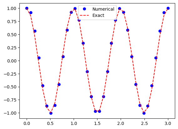
Lets consider the vibration problem as a boundary value problem

\[ u'' + \omega^2 u = 0,\, t \in (0, T) \quad u(0) = u(T) = I. \]

Boundary value problems cannot be solved easily using marching methods, but the linear algebra FD approach is perfect. Lets solve the problem using a central difference for \(n=1, 2, \ldots, N-1\) and specify the solution for \(n=0\) and \(n=N\). For all internal nodes the equation to solve is

\[ \frac{u^{n+1}-2u^n+u^{n-1}}{\Delta t^2} + \omega^2 u^n = 0. \]

The algebraic problem

\[ A \boldsymbol{u} = \boldsymbol{b}, \]

is now, using \(g = 2-\omega^2 \Delta t^2\),

\[\begin{split} \begin{bmatrix} 1 & 0 & 0 & 0 & 0 & 0 & 0 & 0 & 0 \\ 1 & -g & 1 & 0 & 0 & 0 & 0 & 0 & 0 \\ 0 & 1 & -g & 1 & 0 & 0 & 0 & 0 & 0 \\ 0 & 0 & 1 & -g & 1 & 0 & 0 & 0 & 0 \\ 0 & 0 & 0 & 1 & -g & 1 & 0 & 0 & 0 \\ 0 & 0 & 0 & 0 & 1 & -g & 1 & 0 & 0 \\ 0 & 0 & 0 & 0 & 0 & 1 & -g & 1 & 0 \\ 0 & 0 & 0 & 0 & 0 & 0 & 1 & -g & 1 \\ 0 & 0 & 0 & 0 & 0 & 0 & 0 & 0 & 1 \end{bmatrix} \begin{bmatrix} u^0 \\ u^1 \\ u^2 \\ u^3 \\ u^4 \\ u^5 \\ u^6 \\ u^7 \\ u^8 \end{bmatrix} = \begin{bmatrix} I \\ 0 \\ 0 \\ 0 \\ 0 \\ 0 \\ 0 \\ 0 \\ I \end{bmatrix} \end{split}\]

Note

Notice that the matrix contains items both over and under the main diagonal, which characterizes an implicit method. Compare this with the explicit marching method, where all the matrix items were on the main diagonal or below (lower triangular).

Note

We have applied boundary conditions \(u^0=I\) and \(u^N=I\) by modifying the first and last row of \(A\) as well al setting \(b^0=b^N=I\).

All that remains is to implement and solve the linear algebra problem:

T, N, I, w= 3., 35, 1., 2*np.pi
dt = T/N 
g = 2 - w**2*dt**2
A = sparse.diags([1, -g, 1], np.array([-1, 0, 1]), (N+1, N+1), 'lil')
b = np.zeros(N+1)
A[0, :3] = 1, 0, 0    # Fix first row
A[-1, -3:] = 0, 0, 1  # Fix last row
b[0], b[-1] = I, I
u2 = sparse.linalg.spsolve(A.tocsr(), b)
t = np.linspace(0, T, N+1)
plt.plot(t, u2, 'bo', t, I*np.cos(w*t), 'r--')
plt.legend(['Numerical', 'Exact']);

Finite differentiation matrices

Boundary value problems are usually solved using finite difference differentiation matrices and we will now use Taylor expansions more generically in order to obtain these. To this end let us first use the following expansions, three which are forward, and one backward:

\[\begin{split} \begin{align*} (-1)\quad u^{n-1} &= u^n - h u' + \frac{h^2}{2}u'' - \frac{h^3}{6}u''' + \frac{h^4}{24}u'''' - \cdots \\ (1)\quad u^{n+1} &= u^n + h u' + \frac{h^2}{2}u'' + \frac{h^3}{6}u''' + \frac{h^4}{24}u'''' + \cdots \\ (2)\quad u^{n+2} &= u^n + 2h u' + \frac{2 h^2}{1}u'' + \frac{4 h^3}{3}u''' + \frac{2 h^4}{3}u'''' + \cdots \\ (3)\quad u^{n+3} &= u^n + 3h u' + \frac{9 h^2}{2}u'' + \frac{9 h^3}{2}u''' + \frac{27 h^4}{8}u'''' + \cdots \\ \end{align*} \end{split}\]

Remember, \(u^{n+a} = u(t_{n+a})\) and \(t_{n+a} = (n+a)h\) and we use \(h=\Delta t\) for simplicity.

Consider now the central second order finite difference operator \(u''(t_n)\). We can obtain an expression for this by adding equations (-1) and (1)

\[ \begin{equation*} u''(t_n) = \frac{u^{n+1}-2u^n + u^{n-1}}{h^2} + \frac{h^2}{12}u'''' + \end{equation*} \]

The operation can be set up for all \(n\) as a matrix-vector product

\[ \boldsymbol{u}^{(2)} = D^{(2)} \boldsymbol{u}, \]

where we use \(\boldsymbol{u}^{(2)}=(u''(t_n))_{n=0}^{N}\) to represent the finite difference approximation to the second derivative at the \(N+1\) mesh points. The finite difference differentiation matrix is

\[\begin{split} D^{(2)} = \frac{1}{h^2} \begin{bmatrix} ? & ? & ? & ? & ? & ? & ? & ? \\ 1 & -2 & 1 & 0 & 0 & 0 & 0 & \cdots \\ 0 & 1 & -2 & 1 & 0 & 0 & 0 & \cdots \\ \vdots & & & \ddots & & & &\cdots \\ \vdots & 0 & 0 & 0 & 1& -2& 1& 0 \\ \vdots & 0 & 0& 0& 0& 1& -2& 1 \\ ? & ? & ? & ? & ? & ? & ? & ? \\ \end{bmatrix} \end{split}\]

where the first and last rows are open because the stencil in row 0 requires \(u^{-1}\) and for the row \(N\) it requires \(u^{N+1}\). For these two rows we need to use a different stencil.

A first order accurate expression for \(u''\) can be obtained by subtracting 2 times Eq. (1) from Eq. (2), i.e., \((2)-2(1)\):

\[ (2)-2(1): \, u^{n+2} - 2u^{n+1} = -u^n + \frac{h^2}{1}u'' + h^3 u''' + \frac{7 h^4}{12}u'''' + \]

Isolate \(u''\) to obtain

\[ u'' = \frac{u^{n+2}-2u^{n+1}+u^n}{h^2} - h u''' - \frac{7 h^2}{12}u'''' + \]

The error is first order as the first error term is \(-h u'''\).

Can we do better? Yes, of course, just add one more point to the finite difference stencil using Eq. (3). Now to eliminate both \(u'\) and \(u'''\) terms add the three equations as \(-(3) + 4(2) - 5(1)\) (don’t worry about how I know this yet)

\[ -(3)+4(2)-5(1): \, -u^{n+3}+4u^{n+2}-5u^{n+1} = -2 u^n + h^2 u'' - \frac{11 h^4}{12}u'''' + \]

which leads to the second order accurate

\[ u'' = \frac{-u^{n+3} + 4u^{n+2} - 5u^{n+1} + 2u^n}{h^2} + \frac{11 h^2}{12} u'''' + \]

We can now modify our differentiation matrix \(D^{(2)}\) using this one sided (forward) difference for row 0. For the last row, we can derive the same expression, only using points backward in time:

\[\begin{split} D^{(2)} = \frac{1}{h^2}\begin{bmatrix} 2 & -5 & 4 & -1 & 0 & 0 & 0 & 0 \\ 1 & -2 & 1 & 0 & 0 & 0 & 0 & \cdots \\ 0 & 1 & -2 & 1 & 0 & 0 & 0 & \cdots \\ \vdots & & & \ddots & & & &\cdots \\ \vdots & 0 & 0 & 0 & 1& -2& 1& 0 \\ \vdots & 0 & 0& 0& 0& 1& -2& 1 \\ 0 & 0 & 0 & 0 & -1 & 4 & -5 & 2 \\ \end{bmatrix} \end{split}\]

Let us assemble this matrix in Python

N = 8
dt = 0.5
T = N*dt
D2 = sparse.diags([np.ones(N), np.full(N+1, -2), np.ones(N)], np.array([-1, 0, 1]), (N+1, N+1), 'lil')
D2.toarray()

array([[-2.,  1.,  0.,  0.,  0.,  0.,  0.,  0.,  0.],
       [ 1., -2.,  1.,  0.,  0.,  0.,  0.,  0.,  0.],
       [ 0.,  1., -2.,  1.,  0.,  0.,  0.,  0.,  0.],
       [ 0.,  0.,  1., -2.,  1.,  0.,  0.,  0.,  0.],
       [ 0.,  0.,  0.,  1., -2.,  1.,  0.,  0.,  0.],
       [ 0.,  0.,  0.,  0.,  1., -2.,  1.,  0.,  0.],
       [ 0.,  0.,  0.,  0.,  0.,  1., -2.,  1.,  0.],
       [ 0.,  0.,  0.,  0.,  0.,  0.,  1., -2.,  1.],
       [ 0.,  0.,  0.,  0.,  0.,  0.,  0.,  1., -2.]])

Fix the first and last rows

D2[0, :4] = 2, -5, 4, -1
D2[-1, -4:] = -1, 4, -5, 2
D2 *= (1/dt**2) # don't forget h
D2.toarray()*dt**2

array([[ 2., -5.,  4., -1.,  0.,  0.,  0.,  0.,  0.],
       [ 1., -2.,  1.,  0.,  0.,  0.,  0.,  0.,  0.],
       [ 0.,  1., -2.,  1.,  0.,  0.,  0.,  0.,  0.],
       [ 0.,  0.,  1., -2.,  1.,  0.,  0.,  0.,  0.],
       [ 0.,  0.,  0.,  1., -2.,  1.,  0.,  0.,  0.],
       [ 0.,  0.,  0.,  0.,  1., -2.,  1.,  0.,  0.],
       [ 0.,  0.,  0.,  0.,  0.,  1., -2.,  1.,  0.],
       [ 0.,  0.,  0.,  0.,  0.,  0.,  1., -2.,  1.],
       [ 0.,  0.,  0.,  0.,  0., -1.,  4., -5.,  2.]])

If we apply \(D^{(2)}\) to a vector (mesh function) \(\boldsymbol{f} = (f(t_n))_{n=0}^{N}\), we get the second derivative with second order accuracy. Let us try this first with \(f=t^2\).

t = np.linspace(0, N*dt, N+1)
f = t**2
f

array([ 0.  ,  0.25,  1.  ,  2.25,  4.  ,  6.25,  9.  , 12.25, 16.  ])

d2f = D2 @ f
d2f

array([2., 2., 2., 2., 2., 2., 2., 2., 2.])

Try the same, but with only first order accurate edges

D2e = sparse.diags([1, -2, 1], np.array([-1, 0, 1]), (N+1, N+1), 'lil')
D2e[0, :4] = 1, -2, 1, 0
D2e[-1, -4:] = 0, 1, -2, 1
D2e *= (1/dt**2)
D2e @ f

array([2., 2., 2., 2., 2., 2., 2., 2., 2.])

What happened? Why is it still perfect?

The reason is that the error in the stencil

\[ u'' = \frac{u^{n+2}-2u^{n+1}+u^n}{h^2} - h u''' - \frac{7 h^2}{12}u'''' + \]

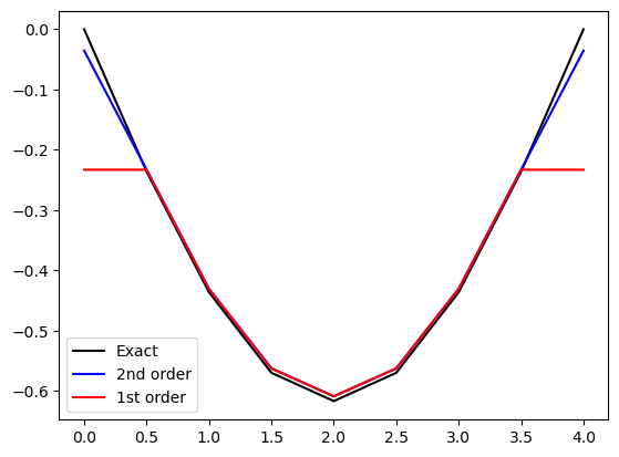
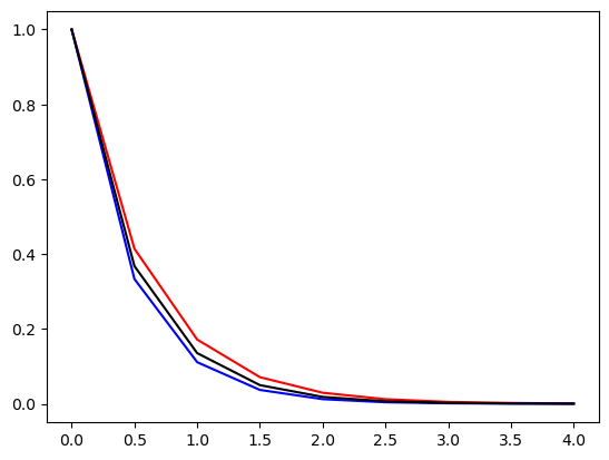
is proportional to \(u'''\), which is 0. Hence we still get no error even though the order is only one. A more complex function would show the error better. Let us try \(f=\sin (\pi t/T)\)

f = np.sin(np.pi*t / T)
d2fe = -(np.pi/T)**2*f
d2f = D2 @ f
d2f1 = D2e @ f
plt.plot(t, d2fe, 'k', t, d2f, 'b', t, d2f1, 'r')
plt.legend(['Exact', '2nd order', '1st order']);

First derivative

Let us create a similar matrix for a first order derivative. We use a central stencil for \(n=1, 2, \ldots N-1\) and skewed stencils for the first and last rows. Again, we need the following Taylor expansions

\[\begin{split} \begin{align} (-1)\quad u^{n-1} &= u^n - h u' + \frac{h^2}{2}u'' - \frac{h^3}{6}u''' + \frac{h^4}{24}u'''' + \cdots \\ (1)\quad u^{n+1} &= u^n + h u' + \frac{h^2}{2}u'' + \frac{h^3}{6}u''' + \frac{h^4}{24}u'''' + \cdots \\ (2)\quad u^{n+2} &= u^n + 2h u' + \frac{2 h^2}{1}u'' + \frac{4 h^3}{3}u''' + \frac{2 h^4}{3}u'''' + \cdots \end{align} \end{split}\]

(1) - (-1) leads to

\[ u'(t_n) = \frac{u^{n+1}-u^{n-1}}{2 h} + \frac{h^2}{6} u''' + \]

We get a first order approximation for \(u'\) using merely Eq. (1):

\[ u'(t_n) = \frac{u^{n+1}-u^n}{h} - \frac{h}{2}u'' - \]

Adding one more equation (Eq. (2)) we get second order: (2)-4(1)

\[ u'(t_n) = \frac{-u^{n+2}+4u^{n+1}-3u^n}{2h} + \frac{h^2}{3}u''' + \]

Hence a second order accurate first differentiation matrix is

\[\begin{split} D^{(1)} = \frac{1}{2 h}\begin{bmatrix} -3 & 4 & -1 & 0 & 0 & 0 & 0 & 0 \\ -1 & 0 & 1 & 0 & 0 & 0 & 0 & \cdots \\ 0 & -1 & 0 & 1 & 0 & 0 & 0 & \cdots \\ \vdots & & & \ddots & & & &\cdots \\ \vdots & 0 & 0 & 0 & -1& 0& 1& 0 \\ \vdots & 0 & 0& 0& 0& -1& 0& 1 \\ 0 & 0 & 0 & 0 & 0 & 1 & -4 & 3 \\ \end{bmatrix} \end{split}\]

D1 = sparse.diags([-1, 1], np.array([-1, 1]), (N+1, N+1), 'lil')
D1[0, :3] = -3, 4, -1
D1[-1, -3:] = 1, -4, 3
D1 *= (1/(2*dt))
D1.toarray()*(2*dt)

array([[-3.,  4., -1.,  0.,  0.,  0.,  0.,  0.,  0.],
       [-1.,  0.,  1.,  0.,  0.,  0.,  0.,  0.,  0.],
       [ 0., -1.,  0.,  1.,  0.,  0.,  0.,  0.,  0.],
       [ 0.,  0., -1.,  0.,  1.,  0.,  0.,  0.,  0.],
       [ 0.,  0.,  0., -1.,  0.,  1.,  0.,  0.,  0.],
       [ 0.,  0.,  0.,  0., -1.,  0.,  1.,  0.,  0.],
       [ 0.,  0.,  0.,  0.,  0., -1.,  0.,  1.,  0.],
       [ 0.,  0.,  0.,  0.,  0.,  0., -1.,  0.,  1.],
       [ 0.,  0.,  0.,  0.,  0.,  0.,  1., -4.,  3.]])

f = t
D1 @ f

array([1., 1., 1., 1., 1., 1., 1., 1., 1.])

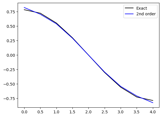
f = np.sin(np.pi*t / T)
d1fe = (np.pi/T)*np.cos(np.pi*t/T)
d1f = D1 @ f
plt.plot(t, d1fe, 'k', t, d1f, 'b')
plt.legend(['Exact', '2nd order'])

<matplotlib.legend.Legend at 0x127c61a90>

Note that D2 is not equal to (D1)^2

D2n = D1 @ D1
D2n.toarray()*dt**2

array([[ 1.25, -2.75,  1.75, -0.25,  0.  ,  0.  ,  0.  ,  0.  ,  0.  ],
       [ 0.75, -1.25,  0.25,  0.25,  0.  ,  0.  ,  0.  ,  0.  ,  0.  ],
       [ 0.25,  0.  , -0.5 ,  0.  ,  0.25,  0.  ,  0.  ,  0.  ,  0.  ],
       [ 0.  ,  0.25,  0.  , -0.5 ,  0.  ,  0.25,  0.  ,  0.  ,  0.  ],
       [ 0.  ,  0.  ,  0.25,  0.  , -0.5 ,  0.  ,  0.25,  0.  ,  0.  ],
       [ 0.  ,  0.  ,  0.  ,  0.25,  0.  , -0.5 ,  0.  ,  0.25,  0.  ],
       [ 0.  ,  0.  ,  0.  ,  0.  ,  0.25,  0.  , -0.5 ,  0.  ,  0.25],
       [ 0.  ,  0.  ,  0.  ,  0.  ,  0.  ,  0.25,  0.25, -1.25,  0.75],
       [ 0.  ,  0.  ,  0.  ,  0.  ,  0.  , -0.25,  1.75, -2.75,  1.25]])

f = np.sin(np.pi*t / T)
d2fe = -(np.pi/T)**2*f
e2 = D2 @ f - d2fe
en = D2n @ f - d2fe
np.sqrt(dt*np.linalg.norm(e2)), np.sqrt(dt*np.linalg.norm(en))

(0.16216463185914778, 0.3704509025277197)

It can be shown that the matrix that is D2n =\(D^{(1)} D^{(1)}\) (matrix product of \(D^{(1)}\) with itself) is only first order accurate.

Solve equations using FD matrices

The FD matrices are great because they depend only on \(h\) and may be implemented once and reused. They only need to be modified in accordance with boundary conditions.

Let’s do the decay equation first and assemble the system

\[ A \boldsymbol{u} = \boldsymbol{b}, \]

for the equation

\[ u' + au = 0, \, t \in (0, T], u(0)=I. \]

Before boundary conditions we can assemble this as

\[ (D^{(1)} + a \mathbb{I})\boldsymbol{u} = \boldsymbol{b}, \]

where \(\mathbb{I}\) is the identity matrix and the only non-zero item in \(\boldsymbol{b}\) is the boundary condition for \(n=0\). We get

\[ \frac{u^{n+1}-u^{n-1}}{2 h} + a u^n = 0. \]

D1 = sparse.diags([-1, 1], np.array([-1, 1]), (N+1, N+1), 'lil')
D1[0, :3] = -3, 4, -1. # Fix boundaries with second order accurate stencil
D1[-1, -3:] = 1, -4, 3
D1 *= (1/(2*dt))
Id = sparse.eye(N+1)
A = D1 + a*Id
b = np.zeros(N+1)
b[0] = I
A[0, :3] = 1, 0, 0 # boundary condition
A.toarray()

array([[ 1.,  0.,  0.,  0.,  0.,  0.,  0.,  0.,  0.],
       [-1.,  2.,  1.,  0.,  0.,  0.,  0.,  0.,  0.],
       [ 0., -1.,  2.,  1.,  0.,  0.,  0.,  0.,  0.],
       [ 0.,  0., -1.,  2.,  1.,  0.,  0.,  0.,  0.],
       [ 0.,  0.,  0., -1.,  2.,  1.,  0.,  0.,  0.],
       [ 0.,  0.,  0.,  0., -1.,  2.,  1.,  0.,  0.],
       [ 0.,  0.,  0.,  0.,  0., -1.,  2.,  1.,  0.],
       [ 0.,  0.,  0.,  0.,  0.,  0., -1.,  2.,  1.],
       [ 0.,  0.,  0.,  0.,  0.,  0.,  1., -4.,  5.]])

u1 = sparse.linalg.spsolve(A, b)
plt.plot(t, u1, 'r', t, u, 'b', t, np.exp(-a*t), 'k');

The scheme is not fully implicit in the source term. However, it is using three neighbouring points for every equation, which is more stable than using merely two.

Generic finite difference stencils

It is possible to derive finite difference stencils of any order from the Taylor expansions around a point in both positive and negative directions. The generic Taylor expansion around \(x=x_0\) reads

\[ u(x) = \sum_{i=0}^{M} \frac{(x-x_0)^i}{i!} u^{(i)}(x_0) + \mathcal{O}((x-x_0)^{M+1}), \]

where \(u^{(i)}(x_0) = \frac{d^{i}u}{dx^{i}}|_{x=x_0}\) and the order of the approximation is \(M+1\).

With the finite difference method we only evaluate this expansion for certain points around \(x_0\). That is, we use only \(x=x_0+ph\), where \(p\) is an integer and \(h\) is a constant (time step or mesh size). We get

\[ u(x_0+ph) = \sum_{i=0}^{M} \frac{(ph)^i}{i!} u^{(i)}(x_0) + \mathcal{O}(h^{M+1}), \]

where we usually use the finite difference notation \(u^{n+p} = u(x_0+ph)\). Note that the equation above is a matrix vector product, because \(\frac{(ph)^i}{i!}\) has two indices \(p, i\) like a matrix and \(u^{(i)}(x_0)\) and \(u(x_0+ph)\) have both only one (\(i\) and \(p\), respectively). With \(c_{pi} = \frac{(ph)^i}{i!}\) and \(du_i = u^{(i)}(x_0)\) and neglecting the \(\mathcal{O}(h^{M+1})\) terms we get

\[ u^{n+p} = \sum_{i=0}^{M} c_{pi} du_i, \]

or in matrix notation

\[ \boldsymbol{u} = C \boldsymbol{du}, \]

where \(\boldsymbol{u} = (u^{n+p})_{p=p_0}^{M+p_0}\), \(C = (c_{p+p_0,i})_{p,i=0}^{M,M}\) and \(\boldsymbol{du}=(du_i)_{i=0}^M\). Here \(p_0\) is an integer representing the lowest value of \(p\) in the stencil.

We can set up a system of equations for \(p_0=-2\) and \(M=4\)

\[\begin{split} \begin{align*} u^{n-2} &= \sum_{i=0}^{M} \frac{(-2h)^i}{i!} du_i \\ u^{n-1} &= \sum_{i=0}^{M} \frac{(-h)^i}{i!} du_i \\ u^{n} &= u^{n} \\ u^{n+1} &= \sum_{i=0}^{M} \frac{(h)^i}{i!} du_i \\ u^{n+2} &= \sum_{i=0}^{M} \frac{(2h)^i}{i!} du_i \\ \end{align*} \end{split}\]

These 5 equations can be written in matrix form as

\[\begin{split} \begin{bmatrix} u^{n-2}\\ u^{n-1}\\ u^{n}\\ u^{n+1}\\ u^{n+2}\\ \end{bmatrix} = \begin{bmatrix} \frac{(-2h)^0}{0!} & \frac{(-2h)^1}{1!} & \frac{(-2h)^2}{2!} & \frac{(-2h)^3}{3!} & \frac{(-2h)^4}{4!} \\ \frac{(-h)^0}{0!} & \frac{(-h)^1}{1!} & \frac{(-h)^2}{2!} & \frac{(-h)^3}{3!} & \frac{(-h)^4}{4!} \\ 1 & 0 & 0 & 0 & 0 \\ \frac{(h)^0}{0!} & \frac{(h)^1}{1!} & \frac{(h)^2}{2!} & \frac{(h)^3}{3!} & \frac{(h)^4}{4!} \\ \frac{(2h)^0}{0!} & \frac{(2h)^1}{1!} & \frac{(2h)^2}{2!} & \frac{(2h)^3}{3!} & \frac{(2h)^4}{4!} \\ \end{bmatrix} \begin{bmatrix} du_{0} \\ du_1 \\ du_2 \\ du_3 \\ du_4 \end{bmatrix} \end{split}\]

or more easily as

\[ \boldsymbol{u} = C \boldsymbol{du}. \]

Remember that the derivatives \(du_i = u^{(i)}(x_0)\) are what we’re normally interested in. And by assembling the matrix \(C\) we can compute any finite difference scheme (!!) simply through:

\[ \boldsymbol{du} = C^{-1} \boldsymbol{u}. \]

For example, for a second order accurate scheme (with \(p=-1, 0, 1\)) we should have

\[ du_2 = u^{(2)}(x_0) = \frac{u^{n+1}-2u^n+u^{n-1}}{h^2}. \]

Let’s derive this with the approach above. The scheme is central so we use \(m=(-1, 0, 1)\) and second order so use \(M=2\). The \(C\) matrix is then

\[\begin{split} C = \begin{bmatrix} 1 & -h & \frac{h^2}{2} \\ 1 & 0 & 0 \\ 1 & h & \frac{h^2}{2} \end{bmatrix} \end{split}\]

In Python using Sympy:

import sympy as sp
x, h = sp.symbols('x,h')
C = sp.Matrix([[1, -h, h**2/2], [1, 0, 0], [1, h, h**2/2]])
C

\[\begin{split}\displaystyle \left[\begin{matrix}1 & - h & \frac{h^{2}}{2}\\1 & 0 & 0\\1 & h & \frac{h^{2}}{2}\end{matrix}\right]\end{split}\]

Take the inverse

C.inv()

\[\begin{split}\displaystyle \left[\begin{matrix}0 & 1 & 0\\- \frac{1}{2 h} & 0 & \frac{1}{2 h}\\\frac{1}{h^{2}} & - \frac{2}{h^{2}} & \frac{1}{h^{2}}\end{matrix}\right]\end{split}\]

The second order central schemes are found in the last two rows. Row 1 is the first derivative, row 2 the second derivative (i.e., row 1 is \(du_1\) and row 2 \(du_2\)). We can also print out the scheme by computing

\[ \boldsymbol{du} = C^{-1} \boldsymbol{u}. \]

For given order 2 we get

\[ du_2 = \sum_{i=0}^2 c_{2i} u^{n-i-1}. \]

u = sp.Function('u')
coef = sp.Matrix([u(x-h), u(x), u(x+h)])
(C.inv())[2, :] @ coef

\[\displaystyle \left[\begin{matrix}- \frac{2 u{\left(x \right)}}{h^{2}} + \frac{u{\left(- h + x \right)}}{h^{2}} + \frac{u{\left(h + x \right)}}{h^{2}}\end{matrix}\right]\]

We can get any finite difference scheme using all the points that we like. To this end let us create a function that computes the matrix \(C\) given any \(m_0\) and \(N\)

def Cmat(p0, M):
  r"""Return Taylor expansion matrix C

  .. math::

    c_{p0+p, i} = (pi)^{i}/i! \in \mathbb{R}^{M+1 \times M+1}
      
    where p = (p0, p0+1, ..., p0+M) and i = 0, 1, ..., M-1

  Parameters
  ----------
  p0 : int
    The lowest index in the stencil
  M : int
    The shape of the returned matrix is M+1 x M+1

  Returns
  -------
  Matrix of type object and shape M+1 x M+1
  """
  C = np.zeros((M+1, M+1), dtype=object)
  for j, p in enumerate(range(p0, p0+M+1)):
    for i in range(M+1):
      C[j, i] = (p*h)**i / sp.factorial(i) 
  return sp.Matrix(C)

For example, to create a forward difference of the second derivative using inly \(u^n, u^{n+1}\) and \(u^{n+2}\) we can use \(p=0, 1, 2\) and \(M=2\)

\[\begin{split} C = \begin{bmatrix} 1 & 0 & 0 \\ 1 & h & \frac{h^2}{2} \\ 1 & 2h & {2 h^2} \end{bmatrix} \end{split}\]

C = Cmat(0, 2)
coef = sp.Matrix([u(x), u(x+h), u(x+2*h)])
(C.inv())[2, :] @ coef

\[\displaystyle \left[\begin{matrix}\frac{u{\left(x \right)}}{h^{2}} - \frac{2 u{\left(h + x \right)}}{h^{2}} + \frac{u{\left(2 h + x \right)}}{h^{2}}\end{matrix}\right]\]

However, this scheme will only be first order accurate, because it is not central. A second order scheme needs to use one more point, and thus \(p=0,1,2,3\) and \(M=3\)

\[\begin{split} C = \begin{bmatrix} 1 & 0 & 0 & 0 \\ 1 & h & \frac{h^2}{2} & \frac{h^3}{6} \\ 1 & 2h & {2 h^2} & \frac{8 h^3}{6} \\ 1 & 3h & \frac{9 h^2}{2} & \frac{27 h^3}{6} \\ \end{bmatrix} \end{split}\]

C = Cmat(0, 3)
C.inv()

\[\begin{split}\displaystyle \left[\begin{matrix}1 & 0 & 0 & 0\\- \frac{11}{6 h} & \frac{3}{h} & - \frac{3}{2 h} & \frac{1}{3 h}\\\frac{2}{h^{2}} & - \frac{5}{h^{2}} & \frac{4}{h^{2}} & - \frac{1}{h^{2}}\\- \frac{1}{h^{3}} & \frac{3}{h^{3}} & - \frac{3}{h^{3}} & \frac{1}{h^{3}}\end{matrix}\right]\end{split}\]

coef = sp.Matrix([u(x), u(x+h), u(x+2*h), u(x+3*h)])
(C.inv())[2, :] @ coef

\[\displaystyle \left[\begin{matrix}\frac{2 u{\left(x \right)}}{h^{2}} - \frac{5 u{\left(h + x \right)}}{h^{2}} + \frac{4 u{\left(2 h + x \right)}}{h^{2}} - \frac{u{\left(3 h + x \right)}}{h^{2}}\end{matrix}\right]\]

Backward difference:

C = Cmat(-3, 3)
C.inv()

\[\begin{split}\displaystyle \left[\begin{matrix}0 & 0 & 0 & 1\\- \frac{1}{3 h} & \frac{3}{2 h} & - \frac{3}{h} & \frac{11}{6 h}\\- \frac{1}{h^{2}} & \frac{4}{h^{2}} & - \frac{5}{h^{2}} & \frac{2}{h^{2}}\\- \frac{1}{h^{3}} & \frac{3}{h^{3}} & - \frac{3}{h^{3}} & \frac{1}{h^{3}}\end{matrix}\right]\end{split}\]

coef = sp.Matrix([u(x-3*h), u(x-2*h), u(x-h), u(x)])
(C.inv())[1, :] @ coef

\[\displaystyle \left[\begin{matrix}\frac{11 u{\left(x \right)}}{6 h} - \frac{u{\left(- 3 h + x \right)}}{3 h} + \frac{3 u{\left(- 2 h + x \right)}}{2 h} - \frac{3 u{\left(- h + x \right)}}{h}\end{matrix}\right]\]

This is the stencil used for the first and last row of the second derivative matrix for the vibration problem.

Weekly assignments

​This weeks’ assignment is to modify the file VibFD.py, which is containing a test and a vibration equation solver. The solver is implemented as a class in order to experiment easily with different numerical schemes, to be implemented in the __call__ method. The class also contains methods for computing the l2-error and the order of convergence.

The original solver described in the first chapter of Finite Difference Computing with PDEs is implemented in the class VibHPL. In addition to this solver I have created three more solver classes VibFD2, VibFD3 and VibFD4. The first two are second order and the last should be fourth order. The assignment is to implement the __call__ method in these three classes such that the test in test_order will pass. This tests the order of the implemented solvers.

1. For VibFD2 use a central difference scheme

   \[ \frac{u^{n+1}-2u^n+u^{n-1}}{\Delta t^2} + \omega^2 u^{n}=0, \quad n\in (1, 2, \ldots, N-1) \]

   and then use Dirichlet boundary conditions for both sides of the domain: \(u(0)=u(T)=I\), where \(T=N \Delta t\). Dirichlet boundary conditions are set by modifying the first and last rows of the assembled matrix.

2. For VibFD3 use the same central difference scheme, but modify the boundary conditions to: \(u(0)=I\) and u’(T)=0. Here you only need to modify the last row of the assembled matrix from assignment 1.

3. For VibFD4 use a fourth order central difference scheme

   \[ \frac{-u^{n+2} + 16u^{n+1}-30u^{n}+16 u^{n-1}-u^{n-2}}{12\Delta t^2} + \omega^2 u^{n}=0, \quad n\in (2, \ldots, N-2) \]

   For \(n=1\) and \(n=N-1\) use a skewed scheme:

   \[ \frac{u^{n+4}-6 u^{n+3}+14 u^{n+2}- 4u^{n+1}-15 u^{n} + 10 u^{n-1}}{12 \Delta t^2} \]

   and set Dirichlet boundary conditions exactly like in 1. for rows 0 and N.

   Note that it is a little bit more difficult to prove fourth order convergence than second. This is because the error disappears fast, and also because even though the error in the finite difference method is leading fourth order, this does not mean that the fifth order is negligible. And the fifth order error is closer to the fourth than the third order is to the second. So you may need to use higher tolerance (tol) for the test_order function.

4. Finally, we would like to extend the solvers to work for any analytical (manufactured) solution.  To this end we need to solve the vibration equation with a non-zero right hand side

   \[ u''+\omega^2 u = f \]

   where \(f(t)\) will depend on the chosen manufactured solution \(u_e(t)\). Modify the solver VibFD2 such that the modified vibration equation is solved and verify the implementation. It should still be second order accurate. Test using both \(u(t)=t^4\) and \(u(t)=\exp(\sin t)\). Note: do not use a too big domain and set the boundary conditions using the exact \(u(0)\) and \(u(T)\). This way T does not need to be n*pi/w, which is required for the exact cosine solution.

   For this equation you should use sympy, both to set the exact solution and to compute \(f(t)\). The numerical scheme is

   \[ \frac{u^{n+1}-2u^n+u^{n-1}}{\Delta t^2} + \omega^2 u^{n}=f^n, \quad n\in (1, 2, \ldots, N-1) \]

   Note: This assignment is exactly like 1., except that you need to include \(f^n\) in the assembled right hand side vector.

​