3. Suggested solutions weekly assignments - lecture 11

1. Solve the inhomogeneous Helmholtz equation

\[ u'' + \alpha u = f, \quad x \in (-1, 1), u(\pm 1)=0, \]

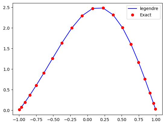
using the manufactured solution \(u(x)=(1-x^2)\exp(\cos(x-0.5))\) and \(\alpha=0.1\). Try also to remove \(1-x^2\) and solve the same problem with inhomogeneous boundary conditions. Plot both the solution and the \(L^2\) error.

Using first shenfun

import matplotlib.pyplot as plt
from shenfun import *
import sympy as sp 
x = sp.Symbol('x')

def solve(N, ue, family='Legendre', alpha=sp.Rational(1, 10)):
    V = FunctionSpace(N, family=family, bc=(ue.subs(x, -1), ue.subs(x, 1)))
    f = ue.diff(x, 2) + alpha*ue 
    u = TrialFunction(V)
    v = TestFunction(V)
    A = inner(Dx(u, 0, 2)+alpha*u, v)
    b = inner(f, v)
    uN = la.Solver(A)(b)
    return uN 

ue = (1-x**2)*sp.exp(sp.cos(x-sp.S.Half))
uN = solve(20, ue)
uj = uN.backward()
xj = uN.function_space().mesh()
plt.plot(xj, uj, 'b', xj, sp.lambdify(x, ue)(xj), 'ro')
plt.legend([uN.function_space().family(), 'Exact']);

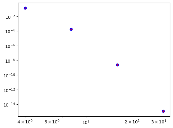
Compute L2-error and plot it to show the spectral accuracy. Both for Legendre and Chebyshev. Note that with Chebyshev shenfun automatically chooses a weighted inner product with weight \(1/\sqrt{1-x^2}\).

def L2_error(uN, ul):
    domain = uN.function_space().domain
    xj = np.linspace(domain[0], domain[1], len(uN)*10)
    uj = uN(xj)
    uej = ul(xj)
    return np.sqrt(np.trapz((uj-uej)**2, dx=xj[1]-xj[0]))

ue = (1-x**2)*sp.exp(sp.cos(x-sp.S.Half))
ul = sp.lambdify(x, ue)
error = {}
for family in ('Chebyshev', 'Legendre'):
    error[family] = []
    for N in 2**np.arange(2, 6):
        uN = solve(N, ue)
        error[family].append(L2_error(uN, ul))

plt.loglog(2**np.arange(2, 6), error['Legendre'], 'bo', 
           2**np.arange(2, 6), error['Chebyshev'], 'r+');

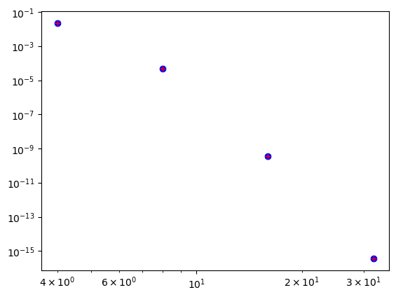
Now do the same thing with inhomogeneous boundary conditions. The accuracy should be approximately the same.

ue = sp.exp(sp.cos(x-sp.S.Half))
ul = sp.lambdify(x, ue)
error2 = {}
for family in ('Chebyshev', 'Legendre'):
    error2[family] = []
    for N in 2**np.arange(2, 6):
        uN = solve(N, ue)
        error2[family].append(L2_error(uN, ul))

plt.loglog(2**np.arange(2, 6), error2['Legendre'], 'bo', 
           2**np.arange(2, 6), error2['Chebyshev'], 'r+');

Note that the solution now contains the boundary conditions. In Shenfun the two boundary conditions of the inhomogeneous Dirichlet space are stored in the last two items of the array of unknowns uN.

uN = solve(20, ue)
print(uN[-2:])

[1.07329913 2.40507854]

The exact boundary values are:

print(ue.subs(x, -1).n(), ue.subs(x, 1).n())

1.07329912758172 2.40507854457258

Now solve the same problem using collocation. Implement by modifying some code from lecture 11.

from lagrange import PolyDerivative
from scipy.interpolate import BarycentricInterpolator 

def Helmholtz_coll(N, f, xj, bc=(0, 0), alpha=0.1):
    D = PolyDerivative(xj, 2)      # Get second derivative matrix
    M = np.eye(N+1)
    A = D + alpha*M
    A[0, 0] = 1; A[0, 1:] = 0      # ident first row
    A[-1, -1] = 1; A[-1, :-1] = 0  # ident last row
    fh = np.zeros(N+1)
    fh[1:-1] = sp.lambdify(x, f)(xj[1:-1])
    fh[0], fh[-1] = bc             # Fix boundary conditions
    uh = np.linalg.solve(A, fh)
    return uh

def l2_error(uh, ul, xj):
    N = len(uh)-1
    L = BarycentricInterpolator(xj, yi=uh)
    N = 4*len(uh)
    xj = np.linspace(xj[0], xj[-1], N+1)
    return np.sqrt(np.trapz((ul(xj)-L(xj).astype(float))**2, dx=2./N))

ue = sp.exp(sp.cos(x-sp.S.Half))
ul = sp.lambdify(x, ue)
alpha = 0.1
f = ue.diff(x, 2) + alpha*ue
bc = ue.subs(x, -1), ue.subs(x, 1)
err = []
for N in 2**np.arange(2, 6):
    xj = np.cos(np.arange(N+1)*np.pi/N)[::-1]
    uh = Helmholtz_coll(N, f, xj, bc=bc, alpha=alpha)
    err.append(l2_error(uh, ul, xj))

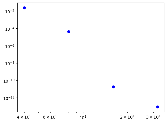
plt.loglog(2**np.arange(2, 6), err, 'bo')

[<matplotlib.lines.Line2D at 0x1349c0740>]

2. Solve the convection-diffusion equation in the domain \(x \in [0, 1]\) and vary the parameter \(\epsilon\) such that \(\epsilon \in (1, 0.1, 0.01, 0.001)\):

\[ u'' + \frac{1}{\epsilon} u' = 0, \quad x \in (0, 1), u(0) = 0, u(1) = 1. \]

The exact solution is here

\[ u(x) = \frac{\exp(-x/\epsilon)-1}{\exp(-1/\epsilon)-1}. \]

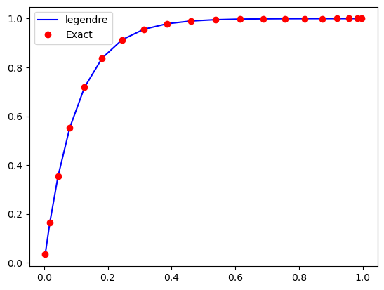
For this problem we create a new shenfun solver, where the right hand side is simply zero. Test first with a relatively large epsilon:

def solveCD(N, ue, family='Legendre', epsilon=sp.Rational(1, 10)):
    V = FunctionSpace(N, family=family, bc=(ue.subs(x, 0), ue.subs(x, 1)), domain=(0, 1))
    u = TrialFunction(V)
    v = TestFunction(V)
    A = inner(Dx(u, 0, 2)+1/epsilon*Dx(u, 0, 1), v)
    b = Function(V)
    uN = la.Solver(A)(b)
    return uN

epsilon = sp.Rational(1, 10)
ue = lambda epsilon: (sp.exp(-x/epsilon)-1) / (sp.exp(-1/epsilon)-1)
uN = solveCD(20, ue(epsilon), epsilon=epsilon.n())
uj = uN.backward()
xj = uN.function_space().mesh()
plt.plot(xj, uj, 'b', xj, sp.lambdify(x, ue(epsilon))(xj), 'ro')
plt.legend([uN.function_space().family(), 'Exact']);

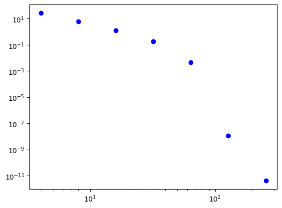
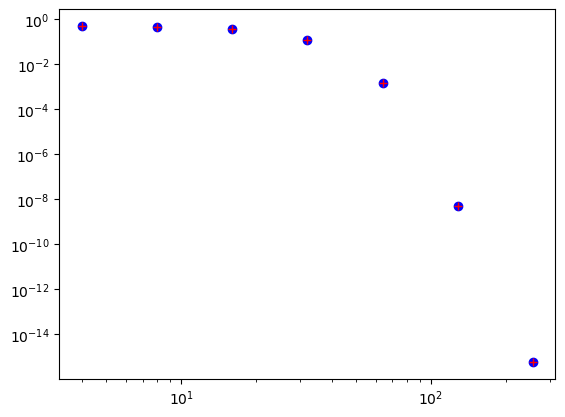
Now check convergence for the most stiff epsilon=1/1000. For this we need quite a few degrees of freedom in order to resolve the sharp gradient of \(u(x)\).

error = {}
epsilon = sp.Rational(1, 1000)
ul = sp.lambdify(x, ue(epsilon))
for family in ('Chebyshev', 'Legendre'):
    error[family] = []
    for N in 2**np.arange(2, 9):
        uN = solveCD(N, ue(epsilon), epsilon=epsilon.n())
        error[family].append(L2_error(uN, ul))

plt.loglog(2**np.arange(2, 9), error['Legendre'], 'bo', 
           2**np.arange(2, 9), error['Chebyshev'], 'r+');

Now solve the same equation using collocation.

def CD_coll(N, xj, bc=(0, 0), epsilon=0.1):
    D2 = PolyDerivative(xj, 2)      # Get second derivative matrix
    D1 = PolyDerivative(xj, 1)      # Get second derivative matrix
    A = D2 + 1/epsilon*D1
    A[0, 0] = 1; A[0, 1:] = 0      # ident first row
    A[-1, -1] = 1; A[-1, :-1] = 0  # ident last row
    fh = np.zeros(N+1)
    fh[0], fh[-1] = bc             # Fix boundary conditions
    uh = np.linalg.solve(A, fh)
    return uh

err = []
for N in 2**np.arange(2, 9):
    xj = (np.cos(np.arange(N+1)*np.pi/N)[::-1]+1)/2 # Get mesh on [0, 1]
    uh = CD_coll(N, xj, bc=(0, 1), epsilon=float(epsilon))
    err.append(l2_error(uh, ul, xj))

plt.loglog(2**np.arange(2, 9), err, 'bo');