MATMEK-4270 presentations – Function approximation by the finite element method

Short recap

We have considered the approximation of functions $u (x), x \in Ω = [a, b]$ using $u (x) \approx u_{N} (x)$ and

$u_{N} (x) = \sum_{i = 0}^{N} {\hat{u}}_{i} ψ_{i} (x)$

$ψ_{i} (x)$ have been global basis functions, defined on all of $Ω = [a, b]$
${{\hat{u}}_{i}}_{i = 0}^{N}$ are the unknowns

We have found ${{\hat{u}}_{i}}_{i = 0}^{N}$ using

The least squares method (variational)
The Galerkin method (variational)
The Collocation method (interpolation)

Advantages and disadvantages of the global variational methods

Advantages

Spectral accuracy
Efficient for orthogonal basis functions
No mesh

Disadvantages

Mainly feasible for simple domains, like lines and rectangles
Inefficient for non-orthogonal basis functions

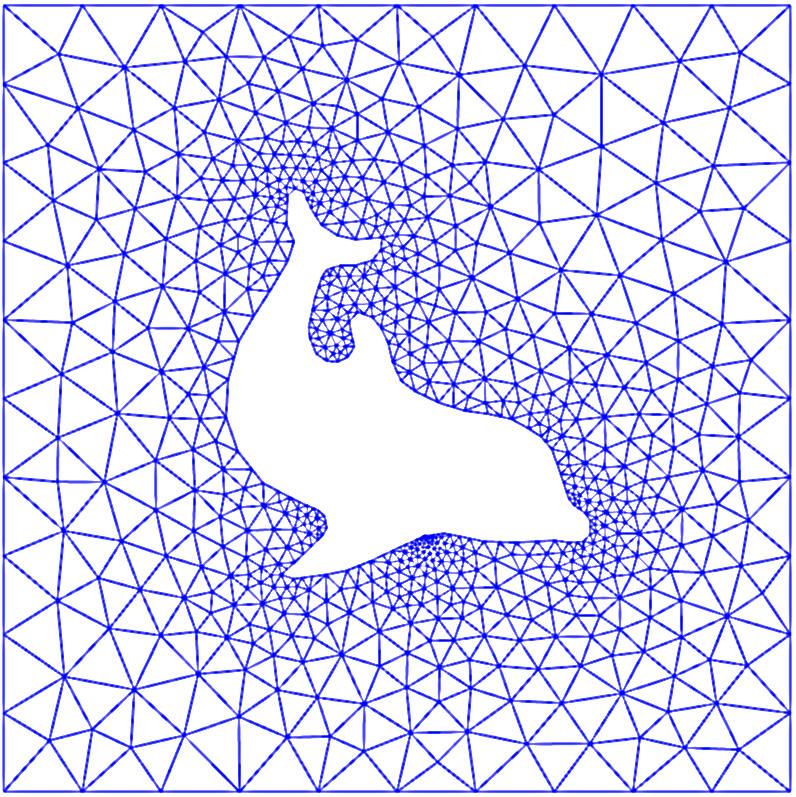
Impossible to use for unstructured meshes, like

The finite element method is a variational method using local basis functions

5 global basis functions

2 local piecewise linear basis functions

The Galerkin formulation is the same whether you use a global approach with Legendre polynomials or a local FEM with piecewise linear polynomials. The difference lies all in the function spaces and the choice of basis.

Find $u_{N} \in V_{N} (= span {ψ_{j}}_{j = 0}^{N})$ such that

$(u - u_{N}, v) = 0 \forall v \in V_{N}$

Piecewise linear basis functions lead to piecewise linear approximations $u_{N} (x)$

With FEM $u_{N} (x)$ is defined everywhere in the domain $Ω$ and not just in mesh points.
Interpolation is not needed since $u_{N} (x) = \sum_{j = 0}^{N} {\hat{u}}_{j} ψ_{j} (x), x \in Ω$ .

The finite element method is especially well suited for unstructured meshes in complex geometries

Structured mesh

Unstructured mesh

But in this course we will learn FEM using simple structured meshes.

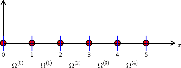
The finite element mesh

The domain $Ω$ is divided into $N_{e}$ smaller, non-overlapping, subdomains $Ω^{(e)}$ , such that

$Ω = ⋃_{e = 0}^{N_{e} - 1} Ω^{(e)}$

The smaller subdomains between the blue lines are referred to as elements.
The red dots are referred to as nodes, just like for interpolation methods.

There may be many nodes inside each element

The figure shows a mesh with 5 non-uniform nodes and 2 non-uniform elements

Using more nodes inside each element is how the FEM can achieve higher order accuracy

Finite element basis functions

An element with no internal nodes can at best use piecewise linear basis functions

$ψ_{j} (x) = {\begin{cases} \frac{x - x_{j - 1}}{x_{j} - x_{j - 1}} & x \in [x_{j - 1}, x_{j}], \\ \frac{x - x_{j + 1}}{x_{j} - x_{j + 1}} & x \in [x_{j}, x_{j + 1}], \\ 0 & otherwise, \end{cases}$

The FEM is a variational method

Use a continuous piecewise linear function space $V_{N} = span {ψ_{j}}_{j = 0}^{N}$ , where

$ψ_{j} (x) = {\begin{cases} \frac{x - x_{j - 1}}{x_{j} - x_{j - 1}} & x \in [x_{j - 1}, x_{j}] \\ \frac{x - x_{j + 1}}{x_{j} - x_{j + 1}} & x \in [x_{j}, x_{j + 1}] \\ 0 & otherwise \end{cases}$

To approximate a function $u (x), x \in Ω = [a, b]$ , we can now use the variational Galerkin method: Find $u_{N} \in V_{N}$ such that

$(u - u_{N}, v) = 0 \forall v \in V_{N}$

We can still use $v = ψ_{i}$ and $u_{N} (x) = \sum_{j = 0}^{N} {\hat{u}}_{j} ψ_{j} (x)$ , exactly like for the global Galerkin method and obtain:

$\sum_{j = 0}^{N} (ψ_{j}, ψ_{i}) {\hat{u}}_{j} = (u, ψ_{i}), i = 0, 1, \dots, N$

The element mass matrix

The mass matrix $A = (a_{i j})_{i, j = 0}^{N}$ is

$a_{i j} = (ψ_{j}, ψ_{i}) = \int_{Ω} ψ_{j} ψ_{i} d x, (i, j) \in (0, \dots, N)^{2}$

However, since each basis function is only non-zero on at most two elements, we usually assemble elementwise and add up (this works very well on unstructured meshes!)

$a_{i j} = \sum_{e = 0}^{N_{e} - 1} a_{i j}^{(e)} = \sum_{e = 0}^{N_{e} - 1} \int_{Ω^{(e)}} ψ_{j} ψ_{i} d x$

We define the element mass matrix $A^{(e)} = (a_{i j}^{(e)})_{i, j = 0}^{N}$ as

$a_{i j}^{(e)} = \int_{Ω^{(e)}} ψ_{j} ψ_{i} d x, (i, j) \in (0, \dots, N)^{2}$

The finite element method is much more difficult to implement than global methods, because of the local basis functions and unstructured mesh. Yet, the unstructured mesh and local basis functions make the method much more flexible.

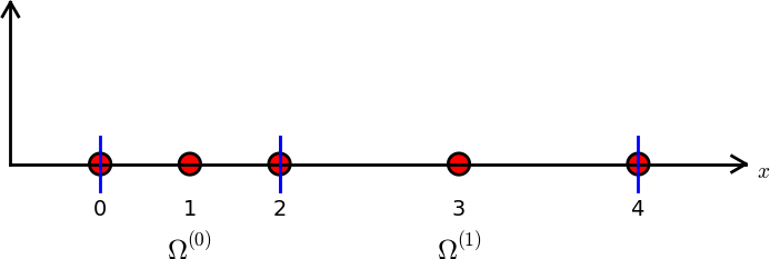
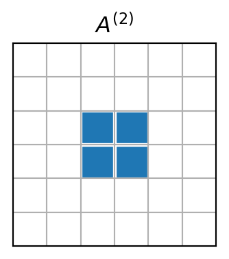
The element mass matrix is highly sparse

$a_{i j}^{(e)} = \int_{Ω^{(e)}} ψ_{j} ψ_{i} d x,$

For piecewise linear basis functions there are only 2 non-zero basis functions per element. See element $Ω^{(2)}$

The matrix $A^{(2)}$ will have only 4 non-zero items. So it is really a waste of memory using an $(N + 1) \times (N + 1)$ matrix.

Define a local-to-global map $q (e, r)$

$q (e, r) = d e + r$

Mapping local index $r \in (0, \dots, d)$ on global element $e$ to the global index $q (e, r) \in (0, 1, \dots, N)$ . There are $d + 1$ nodes per element.

For unstructured meshed $q (e, r)$ needs to be stored explicitly ( $r$ numbering is implicit):

$q = {\begin{matrix} 0 : [\begin{matrix} 0 \\ 1 \\ 2 \end{matrix}] & 1 : [\begin{matrix} 2 \\ 3 \\ 4 \end{matrix}] & 2 : [\begin{matrix} 4 \\ 5 \\ 6 \end{matrix}] \end{matrix}}$

Use a local dense element mass matrix

With $d + 1$ nonzero basis functions on element $e$ all the non-zero items of $A^{(e)}$ can be stored in the dense matrix:

${\tilde{A}}^{(e)} = ({\tilde{a}}_{r s}^{(e)})_{r, s = 0}^{d}$

${\tilde{a}}_{r s}^{(e)} = \int_{Ω^{(e)}} ψ_{q (e, r)} ψ_{q (e, r)} d x$

Note

The matrix ${\tilde{A}}^{(e)}$ contains the same nonzero items as $A^{(e)}$ , but ${\tilde{A}}^{(e)} \in R^{(d + 1) \times (d + 1)}$ is dense, whereas $A^{(e)} \in R^{(N + 1) \times (N + 1)}$ is highly sparse.

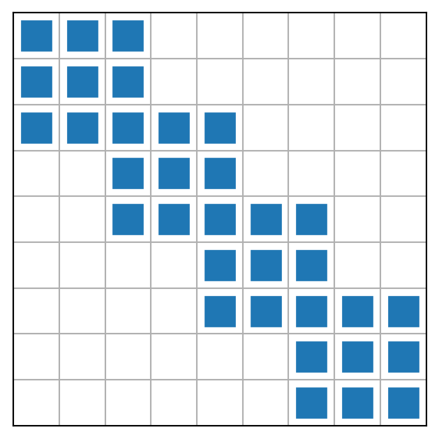
Local to global mapping in assembly of $A$

The 4 smaller matrices represent ${\tilde{A}}^{(0)}, {\tilde{A}}^{(1)}, {\tilde{A}}^{(2)}$ and ${\tilde{A}}^{(3)}$

Finite element assembly: add up for $e = 0, 1, \dots, N_{e} - 1$ and $(r, s) \in (0, 1, \dots, d)^{2}$

$a_{q (e, r), q (e, s)} + = {\tilde{a}}_{r, s}^{(e)}$

Mapping to reference domain

In assembling the matrix $A$ we need to compute the element matrix ${\tilde{A}}^{(e)}$ many times. Is this really necessary? The integrals

$\int_{Ω^{(e)}} ψ_{q (e, r)} ψ_{q (e, s)} d Ω,$

differ only in the domain, whereas the shape of the basis functions is the same regardless of domain. The piecewise linear basis functions are always straight lines.

Let us map all elements to a reference domain $Ω^{r} = [- 1, 1]$ . The affine map from $x \in Ω^{(e)} = [x_{q (e, 0)}, x_{q (e, d)}] = [x_{L}, x_{R}]$ to $X \in Ω^{r}$ can be written for any element as

$x = \frac{1}{2} (x_{L} + x_{R}) + \frac{1}{2} (x_{R} - x_{L}) X$

Mapping back and forth is as usual

$X (x) or x (X)$

Mapping finite element basis functions

The basis functions $ψ_{q (e, r)} (x)$ are commonly mapped to the Lagrangian basis functions

$ψ_{q (e, r)} (x) = ℓ_{r} (X) = \prod_{\begin{matrix} 0 \leq s \leq d \\ s \neq r \end{matrix}} \frac{X - X_{s}}{X_{r} - X_{s}}$

where

$X_{r} = - 1 + \frac{2 r}{d}, r = 0, 1, \dots, d$

and for piecewise linear basis functions ( $d = 1$ ) we get the following basis functions on the reference domain:

$ℓ_{0} (X) = \frac{1}{2} (1 - X) and ℓ_{1} (X) = \frac{1}{2} (1 + X)$

Quadratic elements ( $d = 2$ )

For quadratic elements the Lagrange basis functions on the reference domain are

$(X_{0}, X_{1}, X_{2}) = (- 1, 0, 1)$

$ℓ_{0} (X) = \frac{1}{2} X (1 - X), ℓ_{1} (X) = (1 - X^{2}), ℓ_{2} (X) = \frac{1}{2} X (1 + X)$

d=3 and $(X_{0}, X_{1}, X_{2}, X_{3}) = (- 1, - 1 / 3, 1 / 3, 1)$

$\begin{matrix} ℓ_{0} (X) = - \frac{9}{16} (X - 1) (X - \frac{1}{3}) (X + \frac{1}{3}) & ℓ_{1} (X) = \frac{27}{16} (X - 1) (X - \frac{1}{3}) (X + 1) \\ ℓ_{2} (X) = - \frac{27}{16} (X - 1) (X + \frac{1}{3}) (X + 1) & ℓ_{3} (X) = \frac{9}{16} (X - \frac{1}{3}) (X + \frac{1}{3}) (X + 1) \end{matrix}$

Back to the element matrix

Use a change of variables ( $x \to X$ and $ψ_{q (e, r)} (x) = ℓ_{r} (X)$ ) for the inner product:

$\begin{aligned} {\tilde{a}}_{r s}^{(e)} & = \int_{Ω^{(e)}} ψ_{q (e, r)} (x) ψ_{q (e, s)} (x) d Ω, \\ = \int_{x_{L}}^{x_{R}} ψ_{q (e, r)} (x) ψ_{q (e, s)} (x) d x, \\ = \int_{- 1}^{1} ℓ_{r} (X) ℓ_{s} (X) \frac{d x}{d X} d X, \end{aligned}$

where $d x / d X = h (e) / 2$ and $h (e) = x_{q (e, d)} - x_{q (e, 0)} = x_{R} - x_{L}$ , such that for any element, regardless of order $d$ , we can compute the elements of the element matrix as

${\tilde{a}}_{r s}^{(e)} = \frac{h (e)}{2} \int_{- 1}^{1} ℓ_{r} (X) ℓ_{s} (X) d X$

Note that the integral does not depend on element number $e$ !

Since the integral does not depend on the element

then, instead of computing for each (linear) element:

${\tilde{A}}^{(e)} = [\begin{matrix} \int_{Ω^{(e)}} ψ_{q (e, 0)} ψ_{q (e, 0)} d x & \int_{Ω^{(e)}} ψ_{q (e, 0)} ψ_{q (e, 1)} d x \\ \int_{Ω^{(e)}} ψ_{q (e, 1)} ψ_{q (e, 0)} d x & \int_{Ω^{(e)}} ψ_{q (e, 1)} ψ_{q (e, 1)} d x \end{matrix}],$

we can simply use:

${\tilde{A}}^{(e)} = \frac{h (e)}{2} [\begin{matrix} \int_{- 1}^{1} ℓ_{0} ℓ_{0} d X & \int_{- 1}^{1} ℓ_{0} ℓ_{1} d X \\ \int_{- 1}^{1} ℓ_{1} ℓ_{0} d X & \int_{- 1}^{1} ℓ_{1} ℓ_{1} d X \end{matrix}] .$

with merely a different $h (e)$ for each element.

Similarly for higher $d$ .

Sympy implementation element mass matrix

Linear ( $d = 1$ )

h = sp.Symbol('h')
l = Lagrangebasis([-1, 1])
ae = lambda r, s: sp.integrate(l[r]*l[s], (x, -1, 1))
A1e = h/2*sp.Matrix([[ae(0, 0), ae(0, 1)],[ae(1, 0), ae(1, 1)]])
A1e

$[\begin{matrix} \frac{h}{3} & \frac{h}{6} \\ \frac{h}{6} & \frac{h}{3} \end{matrix}]$

Quadratic ( $d = 2$ )

l = Lagrangebasis([-1, 0, 1])
ae = lambda r, s: sp.integrate(l[r]*l[s], (x, -1, 1))
A2e = h/2*sp.Matrix(np.array([[ae(i, j) for i in range(3) for j in range(3)]]).reshape(3, 3))
A2e

$[\begin{matrix} \frac{2 h}{15} & \frac{h}{15} & - \frac{h}{30} \\ \frac{h}{15} & \frac{8 h}{15} & \frac{h}{15} \\ - \frac{h}{30} & \frac{h}{15} & \frac{2 h}{15} \end{matrix}]$

Complete assembly implementation

Ae = [A1e, A2e] # previously computed

def get_element_boundaries(xj, e, d=1):
    return xj[d*e], xj[d*(e+1)]

def get_element_length(xj, e, d=1):
    xL, xR = get_element_boundaries(xj, e, d=d)
    return xR-xL

def local_to_global_map(e, r=None, d=1): # q(e, r)
    if r is None:
        return slice(d*e, d*(e+1)+1)
    return d*e+r

def assemble_mass(xj, d=1):
    N = len(xj)-1
    Ne = N//d
    A = np.zeros((N+1, N+1))
    for elem in range(Ne):
        hj = get_element_length(xj, elem, d=d)
        s0 = local_to_global_map(elem, d=d)
        A[s0, s0] += np.array(Ae[d-1].subs(h, hj), dtype=float)
    return A

N = 4
xj = np.linspace(1, 2, N+1)
A = assemble_mass(xj, d=1)
print(A)

[[0.0833 0.0417 0.     0.     0.    ]
 [0.0417 0.1667 0.0417 0.     0.    ]
 [0.     0.0417 0.1667 0.0417 0.    ]
 [0.     0.     0.0417 0.1667 0.0417]
 [0.     0.     0.     0.0417 0.0833]]

Higher order mass matrix

N = 8
xj = np.linspace(1, 2, N+1)
A = assemble_mass(xj, d=2)
print(A)

[[ 0.0333  0.0167 -0.0083  0.      0.      0.      0.      0.      0.    ]
 [ 0.0167  0.1333  0.0167  0.      0.      0.      0.      0.      0.    ]
 [-0.0083  0.0167  0.0667  0.0167 -0.0083  0.      0.      0.      0.    ]
 [ 0.      0.      0.0167  0.1333  0.0167  0.      0.      0.      0.    ]
 [ 0.      0.     -0.0083  0.0167  0.0667  0.0167 -0.0083  0.      0.    ]
 [ 0.      0.      0.      0.      0.0167  0.1333  0.0167  0.      0.    ]
 [ 0.      0.      0.      0.     -0.0083  0.0167  0.0667  0.0167 -0.0083]
 [ 0.      0.      0.      0.      0.      0.      0.0167  0.1333  0.0167]
 [ 0.      0.      0.      0.      0.      0.     -0.0083  0.0167  0.0333]]

Sparsity pattern:

Note

The internal nodes represent rows with only 3 nonzero items. The nodes on the boundary between two elements have rows containing 5 nonzero items.
The mass matrix is not diagonal, but it is sparse.

Finite element assembly of a vector

In solving for

$\sum_{j = 0}^{N} (ψ_{j}, ψ_{i}) {\hat{u}}_{j} = (u, ψ_{i}), i = 0, 1, \dots, N$

we also need the right hand side

$b_{i} = (u, ψ_{i}), i = 0, 1, \dots, N$

This inner product can also be evaluated elementwise, and mapped just like the mass matrix. We define the element vector similarly as the element matrix

$b_{i}^{(e)} = \int_{Ω^{(e)}} u (x) ψ_{i} (x) d x, i = 0, 1, \dots, N$

$b_{i}^{(e)}$ will be highly sparse.

Define a dense local vector

${\tilde{b}}_{r}^{(e)} = (u, ψ_{q (e, r)}) = \int_{Ω^{(e)}} u (x) ψ_{q (e, r)} (x) d x, r = 0, 1, \dots, d$

Using as before $ψ_{q (e, r)} (x) = ℓ_{r} (X)$ we get a mapping to the reference domain

${\tilde{b}}_{r}^{(e)} = \frac{h (e)}{2} \int_{- 1}^{1} u (x (X)) ℓ_{r} (X) d X, r = 0, 1, \dots, d$

Note

The vector ${\tilde{b}}^{(e)}$ needs to be assembled with an integral for each element because of $u (x (X))$

Assemble by adding up for all elements $e = 0, 1, \dots, N_{e} - 1$ and $r = 0, 1, \dots, d$

$b_{q (e, r)} + = {\tilde{b}}_{r}^{(e)}$

Implementation $b^{(e)}$

def map_true_domain(xj, e, d=1, x=x): # return x(X)
    xL, xR = get_element_boundaries(xj, e, d=d)
    hj = get_element_length(xj, e, d=d)
    return (xL+xR)/2+hj*x/2

def map_reference_domain(xj, e, d=1, x=x): # return X(x)
    xL, xR = get_element_boundaries(xj, e, d=d)
    hj = get_element_length(xj, e, d=d)
    return (2*x-(xL+xR))/hj

def map_u_true_domain(u, xj, e, d=1, x=x): # return u(x(X))
    return u.subs(x, map_true_domain(xj, e, d=d, x=x))

def assemble_b(u, xj, d=1):
    l = Lagrangebasis(np.linspace(-1, 1, d+1), sympy=False)
    N = len(xj)-1
    Ne = N//d
    b = np.zeros(N+1)
    for elem in range(Ne):
        hj = get_element_length(xj, elem, d=d)
        us = sp.lambdify(x, map_u_true_domain(u, xj, elem, d=d))
        integ = lambda xj, r: us(xj)*l[r](xj)
        for r in range(d+1):
            b[local_to_global_map(elem, r, d)] += hj/2*quad(integ, -1, 1, args=(r,))[0]
    return bdef map_true_domain(xj, e, d=1, x=x): # return x(X)
    xL, xR = get_element_boundaries(xj, e, d=d)
    hj = get_element_length(xj, e, d=d)
    return (xL+xR)/2+hj*x/2

def map_reference_domain(xj, e, d=1, x=x): # return X(x)
    xL, xR = get_element_boundaries(xj, e, d=d)
    hj = get_element_length(xj, e, d=d)
    return (2*x-(xL+xR))/hj

def map_u_true_domain(u, xj, e, d=1, x=x): # return u(x(X))
    return u.subs(x, map_true_domain(xj, e, d=d, x=x))

def assemble_b(u, xj, d=1):
    l = Lagrangebasis(np.linspace(-1, 1, d+1), sympy=False)
    N = len(xj)-1
    Ne = N//d
    b = np.zeros(N+1)
    for elem in range(Ne):
        hj = get_element_length(xj, elem, d=d)
        us = sp.lambdify(x, map_u_true_domain(u, xj, elem, d=d))
        integ = lambda xj, r: us(xj)*l[r](xj)
        for r in range(d+1):
            b[local_to_global_map(elem, r, d)] += hj/2*quad(integ, -1, 1, args=(r,))[0]
    return b

Note

We need to perform an integral by calling quad for each $r$ in each element.

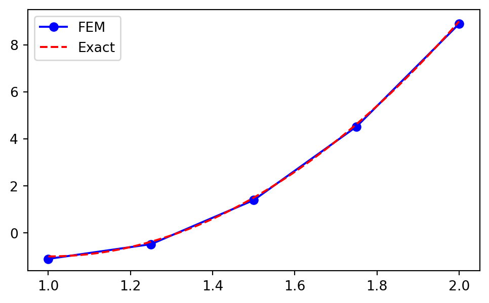
Example: $u (x) = 10 (x - 1)^{2} - 1, x \in [1, 2]$

Use the previously implemented assemble_mass and assemble_b to find the approximation of $u (x)$ using piecewise linear functions and FEM:

def assemble(u, N, domain=(-1, 1), d=1, xj=None):
    mesh = np.linspace(domain[0], domain[1], N+1) if xj is None else xj
    A = assemble_mass(mesh, d=d)
    b = assemble_b(u, mesh, d=d)
    return A, b

N = 4
xj = np.linspace(1, 2, N+1)
A, b = assemble(10*(x-1)**2-1, N, d=1, xj=xj)
uh = np.linalg.inv(A) @ b
yj = np.linspace(1, 2, 1000)
plt.figure(figsize=(6, 3.5))
plt.plot(xj, uh, 'b-o', yj, 10*(yj-1)**2-1, 'r--')
plt.legend(['FEM', 'Exact']);

Note

Since we are using piecewise linear polynomials we can simply plot uh = $(u_{N} (x_{i}))_{i = 0}^{N} = ({\hat{u}}_{i})_{i = 0}^{N}$ and matplotlib will correctly fill in a linear profile between the points.
The FEM solution $u_{N} (x_{i}) \neq u (x_{i})$

Second order $(d = 2)$

Check that a non-uniform mesh works as well:

$x_{2 i} = 1 + (\cos (2 π i / N) + 1) / 2 and x_{2 i + 1} = \frac{x_{2 i} + x_{2 (i + 1)}}{2}$

N = 6
xj = np.zeros(N+1)
xj[::2] = 1 + (np.cos(np.arange(N//2+1)*np.pi*2/N)[::-1] + 1)/2
xj[1::2] = 0.5*(xj[:-1:2]+xj[2::2])
A, b = assemble(10*(x-1)**2-1, N, d=2, xj=xj)
uh = np.linalg.inv(A) @ b
yj = np.linspace(1, 2, 1000)
plt.figure(figsize=(6, 4))
plt.plot(xj, uh, '-bo', yj, 10*(yj-1)**2-1, 'r--')
plt.plot(xj[1::2], uh[1::2], 'go')
plt.legend(['FEM 2nd order', 'Exact', 'Internal points']);

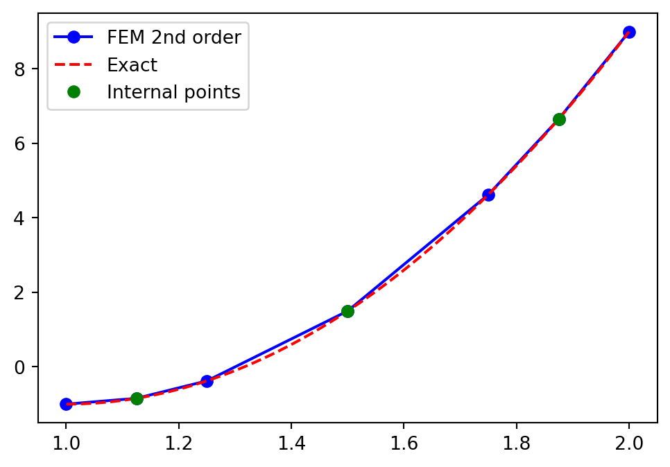
Why still linear interpolation? We need to use the higher order $u_{N} (x) = \sum_{j = 0}^{N} {\hat{u}}_{j} ψ_{j} (x)$ between mesh points! $\to$ FEM evaluation

Finite element evaluation

The finite element solution differs from the finite difference solution in that the solution is automatically defined everywhere within the domain.

$u_{N} (x) = \sum_{j = 0}^{N} {\hat{u}}_{j} ψ_{j} (x)$

However, most basis functions will be zero at any location $x$ . We need to find which element $x$ belongs to! And then evaluate only with non-zero basisfunctions

$u_{N} (x) = \sum_{r = 0}^{d} {\hat{u}}_{q (e, r)} ℓ_{r} (X), x \in Ω^{(e)}$

def fe_evaluate(uh, p, xj, d=1):
    l = Lagrangebasis(np.linspace(-1, 1, d+1), sympy=False)
    elem = max(0, np.argmax(p <= xj[::d])-1) # find element containing p
    Xx = map_reference_domain(xj, elem, d=d, x=p)
    return Lagrangefunction(uh[d*elem:d*(elem+1)+1], l)(Xx)

fe_evaluate(uh, 1.2, xj, d=2), 10*(1.2-1)**2-1

(-0.600000000000000, -0.6000000000000002)

Evaluate FEM for $N_{d}$ points

$u_{N} (x_{i}) = \sum_{r = 0}^{d} {\hat{u}}_{q (e, r)} ℓ_{r} (X (x_{i})), x \in Ω^{(e)}, i = 0, 1, \dots, N_{d} - 1$

Just loop over scalar code for each point

def fe_evaluate_v(uh, pv, xj, d=1):
    uj = np.zeros(len(pv))
    for i, p in enumerate(pv):
        uj[i] = fe_evaluate(uh, p, xj, d)

Alternatively, use vectorization, but not really straightforward:

def fe_evaluate_v(uh, pv, xj, d=1):
    l = Lagrangebasis(np.linspace(-1, 1, d+1), sympy=False)
    # Find points inside elements
    elem = (np.argmax((pv <= xj[::d, None]), axis=0)-1).clip(min=0)
    xL = xj[:-1:d] # All left element boundaries
    xR = xj[d::d]  # All right element boundaries
    xm = (xL+xR)/2 # middle of all elements
    hj = (xR-xL)   # length of all elements
    Xx = 2*(pv-xm[elem])/hj[elem] # map pv to reference space all elements
    dofs = np.array([uh[e*d+np.arange(d+1)] for e in elem], dtype=float)
    V = np.array([lr(Xx) for lr in l], dtype=float) # All basis functions evaluated for all points
    return np.sum(dofs * V.T, axis=1)

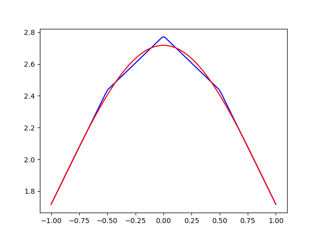
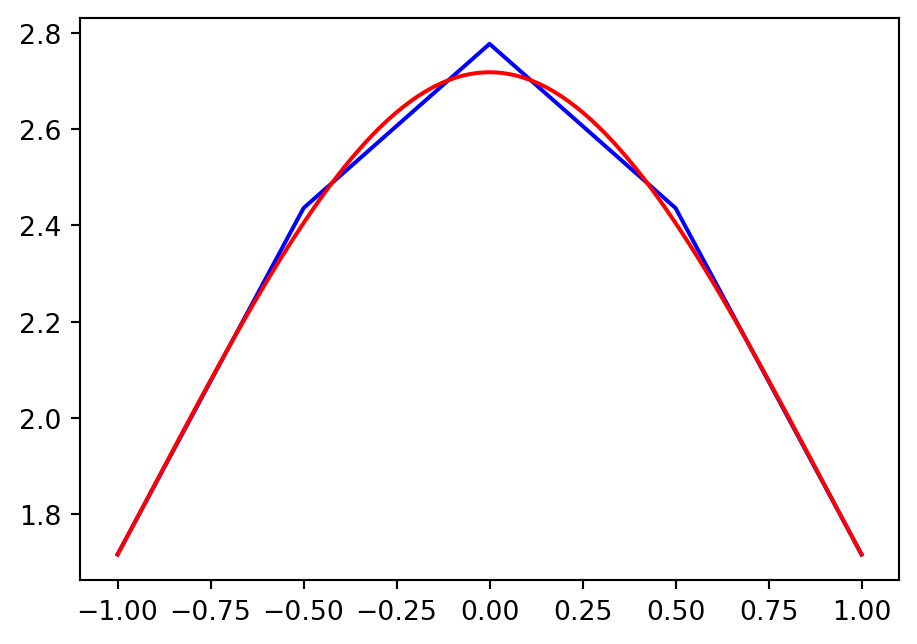
More difficult example: $u (x) = e^{\cos x}$

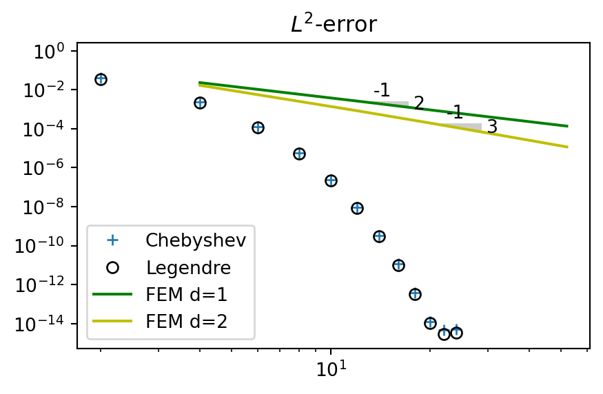
Compute $L^{2} (Ω)$ error and compare with global Chebyshev and Legendre methods

def L2_error(uh, ue, xj, d=1):
    yj = np.linspace(-1, 1, 4*len(xj))
    uhj = fe_evaluate_v(uh, yj, xj, d=d)
    uej = ue(yj)
    return np.sqrt(np.trapz((uhj-uej)**2, dx=yj[1]-yj[0]))

u = sp.exp(sp.cos(x))
ue = sp.lambdify(x, u)
err = []
err2 = []
for n in range(2, 30, 4):
    N = 2*n
    xj = np.linspace(-1, 1, N+1)
    A, b = assemble(u, N, (-1, 1), 1)
    uh = np.linalg.inv(A) @ b
    A2, b2 = assemble(u, N, (-1, 1), 2)
    uh2 = np.linalg.inv(A2) @ b2
    err.append(L2_error(uh, ue, xj, 1))
    err2.append(L2_error(uh2, ue, xj, 2))

Note

This illustrates nicely spectral versus finite order accuracy. With $d = 1$ the FEM obtains second order accuracy and the error disappears as the linear (in the loglog-plot) green curve with slope $- 2$ (from error $\sim N^{- 2}$ ). The spectral error on the other hand disappears exponentially as $\sim e^{- μ N}$ , faster than any finite order.

Finite element software
Developed originally at Chalmers University of Technology and UiO
Very flexible and easy to use
Solves PDEs with many different finite elements, including Lagrange

For installation: https://github.com/FEniCS/dolfinx

Anaconda

conda create -c conda-forge --name fenics fenics-dolfinx mpich pyvista

Linux

sudo add-apt-repository ppa:fenics-packages/fenics
sudo apt update
sudo apt install fenicsx

Docker

docker run -ti dolfinx/dolfinx:stable

First example - function approximation using piecewise linear Lagrange elements

from mpi4py import MPI
from dolfinx import mesh, fem, cpp
from dolfinx.fem.petsc import LinearProblem
import ufl 
from ufl import dx, inner

msh = mesh.create_interval(MPI.COMM_SELF, 4, (-1, 1))
V = fem.functionspace(msh, ("Lagrange", 1))
u = ufl.TrialFunction(V)
v = ufl.TestFunction(V)
xp = ufl.SpatialCoordinate(msh)
ue = ufl.exp(ufl.cos(xp[0]))
a = inner(u, v) * dx
L = inner(ue, v) * dx
problem = LinearProblem(a, L)
uh = problem.solve()

Alternatively assemble and solve linear problem yourself:

from scipy.sparse.linalg import spsolve
A = fem.assemble_matrix(fem.form(a))
b = fem.assemble_vector(fem.form(L))
uh = fem.Function(V)
uh.x.array[:] = spsolve(A.to_scipy(), b.array)

Result 4 piecewise linear basis functions

FEniCS

N = 100
xj = np.zeros((N, 3))
xj[:, 0] = np.linspace(-1, 1, N)
data = cpp.geometry.determine_point_ownership(msh._cpp_object, xj, 1e-8)
plt.plot(xj[:, 0], uh.eval(xj, data.dest_cells), 'b')
plt.plot(xj[:, 0], sp.lambdify(x, sp.exp(sp.cos(x)))(xj[:, 0]), 'r')

Our implementation

N = 4 
A1, b1 = assemble(u, N, (-1, 1), 1)
uN = np.linalg.inv(A1) @ b1
plt.figure(figsize=(5.5, 3.8))
plt.plot(np.linspace(-1, 1, N+1), uN, 'b')
xj = np.linspace(-1, 1, 100)
plt.plot(xj, sp.lambdify(x, u)(xj), 'r')

Exactly the same result for the same method

FEniCS uses exactly the same method with piecewise linear basis functions as we have described using Sympy/Numpy and as such we get exactly the same matrix/vectors:

FEniCS

A.to_dense()

array([[0.1667, 0.0833, 0.    , 0.    , 0.    ],
       [0.0833, 0.3333, 0.0833, 0.    , 0.    ],
       [0.    , 0.0833, 0.3333, 0.0833, 0.    ],
       [0.    , 0.    , 0.0833, 0.3333, 0.0833],
       [0.    , 0.    , 0.    , 0.0833, 0.1667]])

b.array

array([0.4892, 1.1865, 1.3317, 1.1865, 0.4892])

uh.x.array

array([1.7169, 2.4361, 2.7772, 2.4361, 1.7169])

Sympy/Numpy

A1

array([[0.1667, 0.0833, 0.    , 0.    , 0.    ],
       [0.0833, 0.3333, 0.0833, 0.    , 0.    ],
       [0.    , 0.0833, 0.3333, 0.0833, 0.    ],
       [0.    , 0.    , 0.0833, 0.3333, 0.0833],
       [0.    , 0.    , 0.    , 0.0833, 0.1667]])

b1

array([0.4892, 1.1865, 1.3317, 1.1865, 0.4892])

uN

array([1.7169, 2.4361, 2.7772, 2.4361, 1.7169])

Summary

The finite element method (FEM) is a variational method using local basis functions.
The FEM uses the same Galerkin method as the methods using global basis functions.
The FEM is assembled by running over all elements and assembling local matrices and vectors that are subsequently added to global matrices and vectors.
Since all assembly work is performed elementwise, the FEM is very well suited for unstructured meshes.