A simple vibration problem
MATMEK-4270
Prof. Mikael Mortensen, University of Oslo
A simple vibration problem
The vibration equation is given as
\[ u^{\prime\prime}(t) + \omega^2u(t) = 0,\quad u(0)=I,\ u^{\prime}(0)=0,\ t\in (0,T] \]
and the exact solution is:
\[ u(t) = I\cos (\omega t) \]
- \(u(t)\) oscillates with constant amplitude \(I\) and (angular) frequency \(\omega\).
- Period: \(P=2\pi/\omega\). The period is the time between two neighboring peaks in the cosine function.
A centered finite difference scheme; step 1 and 2
Strategy: follow the four steps of the finite difference method.
Step 1: Introduce a time mesh, here uniform on \([0,T]\): \[ t_n=n\Delta t, \quad n=0, 1, \ldots, N_t \]
- Step 2: Let the ODE be satisfied at each mesh point minus 2 boundary conditions:
\[ u^{\prime\prime}(t_n) + \omega^2u(t_n) = 0,\quad n=2,\ldots,N_t \]
A centered finite difference scheme; step 3
Step 3: Approximate derivative(s) by finite difference approximation(s). Very common (standard!) formula for \(u^{\prime\prime}\):
\[ u^{\prime\prime}(t_n) \approx \frac{u^{n+1}-2u^n + u^{n-1}}{\Delta t^2} \]
Insert into vibration ODE:
\[ \frac{u^{n+1}-2u^n + u^{n-1}}{\Delta t^2} = -\omega^2 u^n \]
A centered finite difference scheme; step 4
Step 4: Formulate the computational algorithm. Assume \(u^{n-1}\) and \(u^n\) are known, solve for unknown \(u^{n+1}\):
\[ u^{n+1} = 2u^n - u^{n-1} - \Delta t^2\omega^2 u^n \]
Nick names for this scheme: Störmer’s method or Verlet integration.
The scheme is a recurrence relation. That is, \(u^{n+1}\) is an explicit function of one or more of the solutions at previous time steps \(u^n, u^{n-1}, \ldots\). We will later see implicit schemes where the equation for \(u^{n+1}\) depends also on \(u^{n+2}, u^{n+3}\) etc.
Computing the first step - option 1
- The two initial conditions require that we fix both \(u^0\) and \(u^1\). \(u^0=I\), but how to fix \(u^1\)?
- We cannot use the difference equation \(u^{1} = 2u^0 - u^{-1} - \Delta t^2\omega^2 u^0\) because \(u^{-1}\) is unknown and outside the mesh!
- And: we have to use the initial condition \(u^{\prime}(0)=0\)!
Option 1: Use a forward difference
\[ \begin{align*} u^{\prime}(0) &= \frac{u^1-u^0}{\Delta t}=0 &\longrightarrow u^1=u^0=I \\ u^{\prime}(0) &= \frac{-u^2+4u^1-3u^0}{2 \Delta t}=0 \quad &\longrightarrow u^1=\frac{u^2+3u^0}{4} \end{align*} \]
Note
First is merely first order accurate, second is second order, but implicit (depends on the unknown \(u^2\).)
Computing the first step - option 2
Use the discrete ODE at \(t=0\) together with a central difference at \(t=0\) and a ghost cell \(u^{-1}\). The central difference is
\[ u'(0) \approx \frac{u^1-u^{-1}}{2\Delta t} = 0\quad\Rightarrow\quad u^{-1} = u^1 \]
The vibration scheme for \(n=0\) is
\[ u^{1} = 2u^0 - u^{-1} - \Delta t^2\omega^2 u^0 \]
Use \(u^{-1}=u^1\) to get
\[ u^1 = u^0 - \frac{1}{2} \Delta t^2 \omega^2 u^0 \]
Note
Second order accurate and explicit (does not depend on unknown \(u^2\)).
The computational algorithm
- \(u^0=I\)
- compute \(u^1 = u^0 - \frac{1}{2} \Delta t^2 \omega^2 u^0\)
- for \(n=1, 2, \ldots, N_t-1\):
- compute \(u^{n+1}\)
More precisely expressed in Python:
The code is difficult to vectorize, so we should use Numba or Cython for speed.
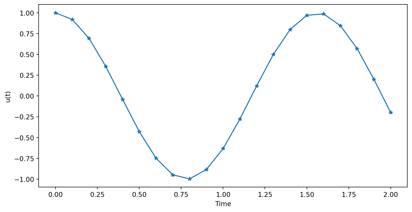
Plot of solution
Computing a numerical \(u^{\prime}\)
\(u\) is often displacement/position, \(u^{\prime}\) is velocity and can be computed by
\[ u^{\prime}(t_n) \approx \frac{u^{n+1}-u^{n-1}}{2\Delta t} \]
Note
For \(u^{\prime}(t_0)\) and \(u^{\prime}(t_{N_t})\) it is possible to use forward or backwards differences, respectively. However, we already know from initial conditions that \(u^{\prime}(t_0) = 0\) so no need to use finite difference there.
Implementation
def solver(I, w, dt, T):
    """
    Solve u'' + w**2*u = 0 for t in (0,T], u(0)=I and u'(0)=0,
    by a central finite difference method with time step dt.
    """
    Nt = int(T/dt)
    u = np.zeros(Nt+1)
    t = np.linspace(0, Nt*dt, Nt+1)

    u[0] = I
    u[1] = u[0] - 0.5*dt**2*w**2*u[0]
    for n in range(1, Nt):
        u[n+1] = 2*u[n] - u[n-1] - dt**2*w**2*u[n]
    return u, t

def u_exact(t, I, w):
    return I*np.cos(w*t)
Visualization
def visualize(u, t, I, w):
    plt.plot(t, u, 'b-o')
    t_fine = np.linspace(0, t[-1], 1001)  # very fine mesh for u_e
    u_e = u_exact(t_fine, I, w)
    plt.plot(t_fine, u_e, 'r--')
    plt.legend(['numerical', 'exact'], loc='upper left')
    plt.xlabel('t')
    plt.ylabel('u(t)')
    dt = t[1] - t[0]
    plt.title('dt=%g' % dt)
    umin = 1.4*u.min();  umax = -umin
    plt.axis([t[0], t[-1], umin, umax])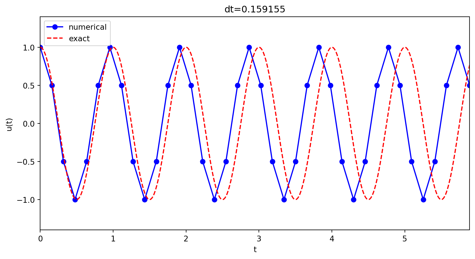
Various timestep

We see that \(\Delta t = 2/\omega\) is a limit. Using longer \(\Delta t\) leads to growth. Why?
Mathematical analysis
The exact solution to the continuous vibration equation is \(u_e(t) = I \cos (\omega t)\)
The key to study the numerical solution is knowing that linear difference equations like
\[ u^{n+1} = (2-\Delta t^2\omega^2) u^n - u^{n-1} \]
admit discrete (numerical) solutions of the form
\[ u^{n+1} = A u^n \quad \text{or} \quad u^n = A^n I \]
where \(I\) is an initial condition.
Exact discrete solution
We now have (at least) two possibilities for \(u^{n+1}=A u^n\)
- Assume that \(A=e^{i \tilde{\omega} \Delta t}\) and solve for the numerical frequency \(\tilde{\omega}\)
- Assume nothing and compute with a function A(\(\Delta t, \omega\)) (like for the exponential decay)
We follow Langtangen’s approach (1) first. Note that since
\[ e^{i \tilde{\omega} \Delta t} = \cos (\tilde{\omega} \Delta t ) + i \sin(\tilde{\omega} \Delta t) \]
we can work with a complex A and let the real part represent the physical solution.
The exact discrete solution is then
\[ u(t_n) = I \cos (\tilde{\omega} t_n) \]
and we can study the error in \(\tilde{\omega}\) compared to the true \(\omega\).
Find the error in \(\tilde\omega\)
Insert the numerical solution \(u^n = I \cos (\tilde{\omega} t_n)\) into the discrete equation
\[ \frac{u^{n+1} - 2u^n + u^{n-1}}{\Delta t^2} + \omega^2 u^n = 0 \]
Quite messy, but Wolfram Alpha (or another long derivation in the FD for PDEs book) will give you for the first FD term
\[ \begin{align} \frac{u^{n+1} - 2u^n + u^{n-1}}{\Delta t^2} &= \frac{I}{\Delta t^2} (\cos (\tilde{\omega} t_{n+1}) - 2 \cos (\tilde{\omega} t_n) + \cos (\tilde{\omega} t_{n-1})) \\ &= \frac{2 I}{\Delta t^2} (\cos (\tilde{\omega} \Delta t) - 1) \cos (\tilde{\omega} n \Delta t) \\ &= -\frac{4}{\Delta t^2} \sin^2 (\tilde{\omega} \Delta t) \cos (\tilde{\omega} n \Delta t) \end{align} \]
Insert into discrete equation
\[ \frac{u^{n+1} - 2u^n + u^{n-1}}{\Delta t^2} + \omega^2 u^n = 0 \]
We get
\[ -\frac{4}{\Delta t^2} \sin^2 (\tilde{\omega} \Delta t) { \cos (\tilde{\omega} n \Delta t)} + { \omega^2 { \cos (\tilde{\omega} n \Delta t)}} = 0 \]
and thus
\[ \omega^2 = \frac{4}{\Delta t^2} \sin^2 \left( \frac{\tilde{\omega} \Delta t}{2} \right) \]
Solve for \(\tilde{\omega}\) by taking the root and using \(\sin^{-1}\)
Numerical frequency
\[ \tilde{\omega} = \pm \frac{2}{\Delta t} \sin^{-1} \left( \frac{\omega \Delta t }{2} \right) \]
- There is always a frequency error because \(\tilde{\omega} \neq \omega\).
- The dimensionless number \(p=\omega\Delta t\) is the key parameter (i.e., no of time intervals per period is important, not \(\Delta t\) itself. Remember \(P=2\pi/w\) and thus \(p=2\pi / P\))
- How good is the approximation \(\tilde{\omega}\) to \(\omega\)?
- Does it possibly lead to growth? \(|A|>1\).
Polynomial approximation of the frequency error
How good is the approximation \(\tilde{\omega} = \pm \frac{2}{\Delta t} \sin^{-1} \left( \frac{\omega \Delta t }{2} \right)\) ?
We can easily use a Taylor series expansion for small \(h=\Delta t\)
So the numerical frequency is always too large (too fast oscillations): \[ \tilde\omega = \omega\left( 1 + \frac{1}{24}\omega^2\Delta t^2\right) + {\cal O}(\Delta t^3) \]
Simple improvement of previous solver
Note
What happens if we simply use the frequency \(\omega(1-\omega^2 \Delta t^2 /24)\) instead of just \(\omega\)?
The leading order numerical error disappears and we get
\[ \tilde\omega = \omega\left( 1 - \left(\frac{1}{24}\omega^2\Delta t^2\right)^2\right) + \cdots \]
Note
Dirty trick, and only usable when you can compute the numerical error exactly. But fourth order…
How about the global error?
\[ u^n = I\cos\left(\tilde\omega n\Delta t\right),\quad \tilde\omega = \frac{2}{\Delta t}\sin^{-1}\left(\frac{\omega\Delta t}{2}\right) \]
The error mesh function,
\[ e^n = u_{e}(t_n) - u^n = I\cos\left(\omega n\Delta t\right) - I\cos\left(\tilde\omega n\Delta t\right) \]
is ideal for verification and further analysis!
\[ \begin{align*} e^n &= I\cos\left(\omega n\Delta t\right) - I\cos\left(\tilde\omega n\Delta t\right) \\ &= -2I\sin\left(n \Delta t\frac{1}{2}\left( \omega - \tilde\omega\right)\right) \sin\left(n \Delta t\frac{1}{2}\left( \omega + \tilde\omega\right)\right) \end{align*} \]
Convergence of the numerical scheme
We can easily show convergence (i.e., \(e^n\rightarrow 0 \hbox{ as }\Delta t\rightarrow 0\)) from what we know about sines in the error
\[ e^n = -2I\sin\left(n \Delta t\frac{1}{2}\left( \omega - \tilde\omega\right)\right) \sin\left(n \Delta t \frac{1}{2}\left( \omega + \tilde\omega\right)\right) \] and the following limit \[ \lim_{\Delta t\rightarrow 0} \tilde\omega = \lim_{\Delta t\rightarrow 0} \frac{2}{\Delta t}\sin^{-1}\left(\frac{\omega\Delta t}{2}\right) = \omega \]
The limit can be computed using L’Hopital’s rule or simply by asking sympy or WolframAlpha. Sympy is easier:
How about stability?
Solutions are oscillatory, so not a problem that \(A<0\), like for the exponential decay
Solutions should have constant amplitudes (constant \(I\)), but we will have growth if \[ |A| > 1 \]
Constant amplitude requires \[ |A| = |e^{i \tilde{\omega} \Delta t}| = 1 \] Is this always satisfied?
Stability in growth?
Consider \[ |A| = |e^{i y}| \quad \text{where} \quad y= \tilde{\omega} \Delta t = \pm 2 \sin^{-1}\left(\frac{\omega \Delta t}{2}\right) \]
Is \(|e^{iy}|=1\) for all \(y\)?
How can we get negative \(\Im(y)\)? Can \(\Im(\sin^{-1}(x)) < 0\) for some \(x\)?
Yes! We can easily check that if \(|x|>1\) then \(\sin^{-1}(x)\) has a negative imaginary part:
Hence if \(\left| \frac{\omega \Delta t}{2} \right| > 1\) then we will have growth! For stability \(\longrightarrow \Delta t \le 2 / w\) !
Stability limit
Summary: we get
\[ \left|\sin^{-1}\left(\frac{\omega \Delta t}{2} \right) \right| > 1 \]
if
\[ \left| \frac{\omega \Delta t}{2} \right| > 1 \]
This happens for
\[ \Delta t > \frac{2}{\omega} \]
Remember the initial plots
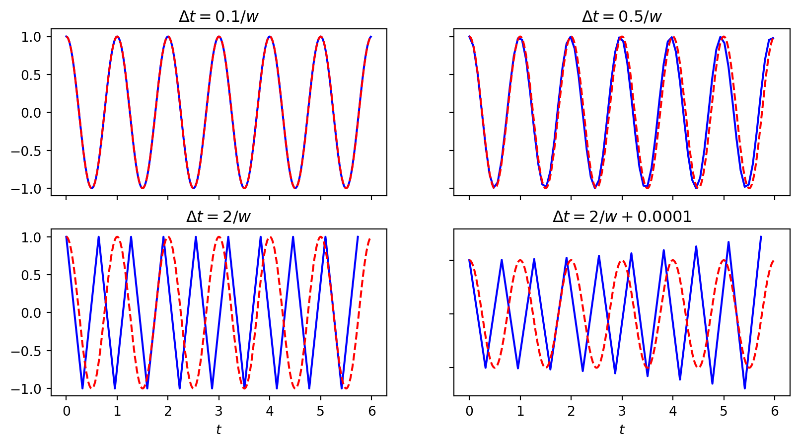
We have growth for \(\Delta t > 2/\omega\).
About the stability limit
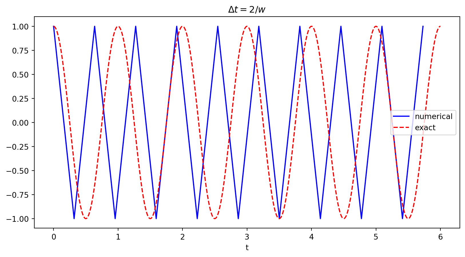
For \(\Delta t = 2/\omega\) there is exactly one timestep between a minimum and a maximum point for the numerical simulation (zigzag pattern). This is absolutely the smallest number of points that can possibly resolve (poorly) a wave of this frequency! So it really does not make sense physically to use larger time steps!
Alternative derivation of stability limit
We have the difference equation
\[ u^{n+1} = (2-\Delta t^2\omega^2) u^n - u^{n-1} \]
and a numerical solution of the form
\[ u^{n} = A^n I \]
Insert for the numerical solution in the difference equation:
\[ A^{n+1}I = (2-\Delta t^2 \omega^2) A^n I - A^{n-1}I \]
Divide by \(I A^{n-1}\) and rearrange
\[ A^2 - (2-\Delta t^2 \omega^2)A + 1 = 0 \]
Alternative derivation ct’d
Set \(p=\Delta t \omega\) and solve second order equation
\[ A = 1 - \frac{p^2}{2} \pm \frac{p}{2}\sqrt{p^2-4} \]
We still want \(|A|=1\) for constant amplitude and stability. However try \(p > 2\) in the above equation (using the minus in front of the last term) and you get
\[ A < -1 \]
Check:
Alternative derivation ct’d
Set \(p=\Delta t \omega\) and solve second order equation
\[ A = 1 - \frac{p^2}{2} \pm \frac{p}{2}\sqrt{p^2-4} \]
We still want \(|A|=1\) for constant amplitude and stability. However try \(p > 2\) in the above equation (using the minus in front of the last term) and you get
\[ A < -1 \]
So we have growth if \(p > 2\), which is the same as \(\Delta t \omega > 2\) or simply
\[ \Delta t > \frac{2}{\omega} \]
which is the same result as we got using the numerical frequency \(\tilde{\omega}\)!
Digression
Digression
This alternative analysis is no different from what we did with the exponential decay. Only the exponential decay was so easy that we did not actually derive the generic A!
Consider the difference equation for exponential decay
\[ \frac{u^{n+1}-u^{n}}{\triangle t} = -(1-\theta)au^{n} - \theta a u^{n+1} \]
and assume again that \(u^n = A^n I\). Insert this into the above
\[ \frac{A^{n+1}I-A^{n}I}{\triangle t} = -(1-\theta)aA^{n}I - \theta a A^{n+1}I \]
Divide by \(A^n I\) and rearrange to get the well-known \(A = \frac{1-(1-\theta)\Delta t a}{1+ \theta \Delta t a}\)
Key observations
We can draw three important conclusions:
- The key parameter in the formulas is \(p=\omega\Delta t\) or \(\tilde{p} = \tilde{\omega} \Delta t\) (dimensionless)
- Period of oscillations: \(P=2\pi/\omega\) vs numerical \(\tilde{P}=2 \pi / \tilde{\omega}\)
- Number of time steps per period: \(N_P=P/\Delta t\) vs \(\tilde{N}_P =\tilde{P}/\Delta t\)
- At stability limit \(\omega = 2/\Delta t\) and \(\tilde{\omega}=\pi/\Delta t\) \(\Rightarrow P = \pi \Delta t\) and \(\tilde{P} = 2 \Delta t\). We get \(\tilde{N}_P = \tilde{P}/\Delta t = 2\) and the critical parameter is really the number of time steps per numerical period.
- For \(p\leq 2\) the amplitude of \(u^n\) is constant (stable solution)
- \(u^n\) has a relative frequency error \(\tilde\omega/\omega \approx 1 + \frac{1}{24}p^2\), making numerical peaks occur too early. This is also called a phase error, or a dispersive error.
Convergence rates
Lets compute the convergence rate for our solver. However, let it also be possible to choose the numerical frequency \(\omega(1-\omega^2\Delta t^2/24)\)
def solver_adjust(I, w, dt, T, adjust_w=False):
    Nt = int(round(T/dt))
    u = np.zeros(Nt+1)
    t = np.linspace(0, Nt*dt, Nt+1)
    w_adj = w*(1 - w**2*dt**2/24.) if adjust_w else w
    u[0] = I
    u[1] = u[0] - 0.5*dt**2*w_adj**2*u[0]
    for n in range(1, Nt):
        u[n+1] = 2*u[n] - u[n-1] - dt**2*w_adj**2*u[n]
    return u, t

def u_exact(t, I, w):
    return I*np.cos(w*t)

def l2_error(dt, T, w=0.35, I=0.3, adjust_w=False):
    u, t = solver_adjust(I, w, dt, T, adjust_w)
    ue = u_exact(t, I, w)
    return np.sqrt(dt*np.sum((ue-u)**2))
Convergence rates
We compute the order of the convergence in the same manner as lecture 2
\[ r = \frac{\log {\frac{E_{i-1}}{E_i}}}{\log {\frac{\Delta t_{i-1}}{\Delta t_i}}} \]
def convergence_rates(m, num_periods=8, w=0.35, I=0.3, adjust_w=False):
    P = 2*np.pi/w
    dt = 1 / w    # Half stability limit
    T = P*num_periods
    dt_values, E_values = [], []
    for i in range(m):
        E = l2_error(dt, T, w, I, adjust_w)
        dt_values.append(dt)
        E_values.append(E)
        dt = dt/2.
    # Compute m-1 orders that should all be the same
    r = [np.log(E_values[i-1]/E_values[i])/
         np.log(dt_values[i-1]/dt_values[i])
         for i in range(1, m, 1)]
    return r, E_values, dt_values
Try it!
Print the computed convergence rates
[np.float64(1.9487030166752326),
 np.float64(2.022988970233581),
 np.float64(2.0050238810553545),
 np.float64(2.0013403129395835)]
Adjusted solver:
plot convergence regular solver
from plotslopes import slope_marker
r, E, dt = convergence_rates(5)
plt.loglog(dt, E, dt, 10*np.array(dt), dt, np.array(dt)**2)
plt.title('Convergence of finite difference method')
plt.legend(['Error', '$\\mathcal{O}(\\Delta t)$', '$\\mathcal{O}(\\Delta t^2)$'])
slope_marker((dt[1], E[1]), (2,1))
slope_marker((dt[1], 10*dt[1]), (1,1))
slope_marker((dt[1], dt[1]**2), (2,1))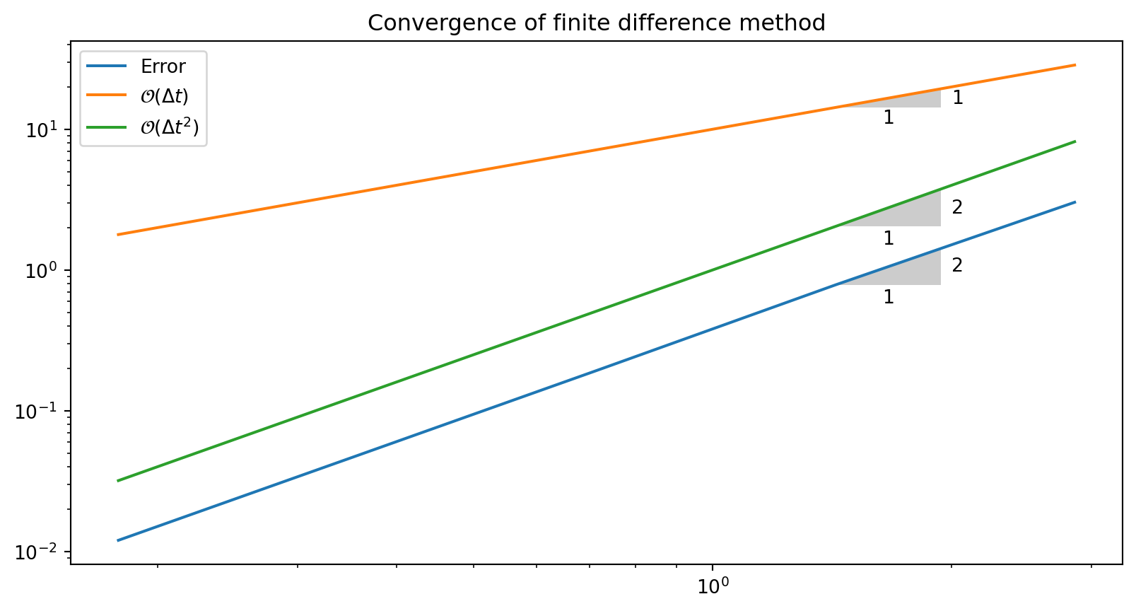
plot convergence adjusted solver
from plotslopes import slope_marker
r, E, dt = convergence_rates(5, adjust_w=True)
plt.loglog(dt, E, dt, np.array(dt)**4)
plt.title('Convergence of finite difference method')
plt.legend(['Error', '$\\mathcal{O}(\\Delta t^4)$'])
slope_marker((dt[1], E[1]), (4,1))
slope_marker((dt[1], dt[1]**4), (4,1))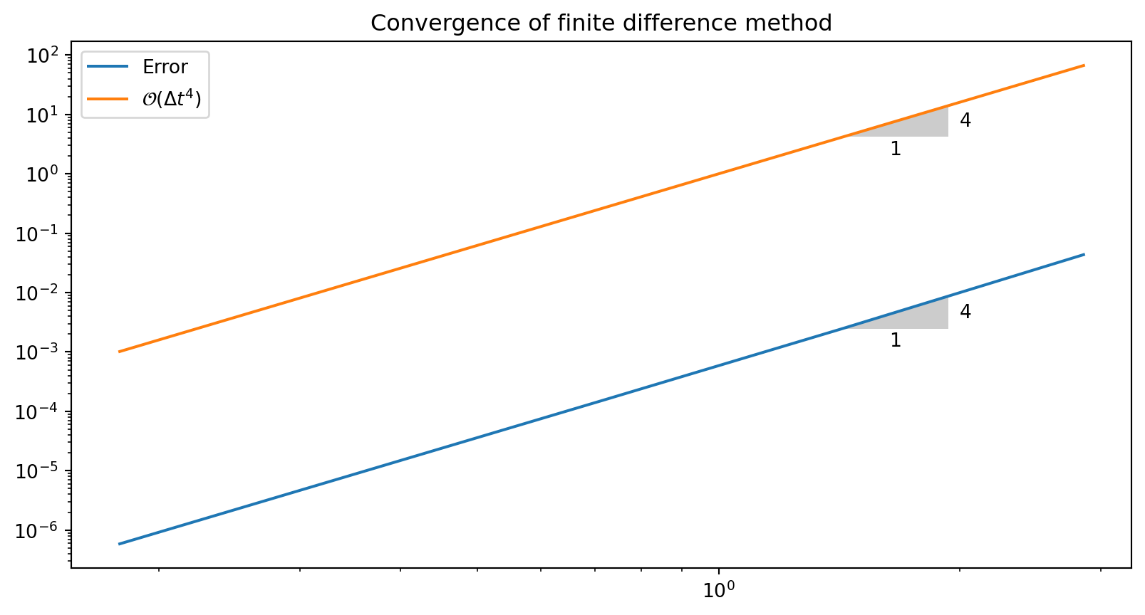
Add tests
The exact solution will not equal the numerical, but the order of the error is something we can test for.
Run test for \(m=4\) levels, \(w=0.5, I=1\) and adjust_w=False
Final test
Use simply an assert clause and do not catch the error.
This test will work with pytest.