import numpy as np
def solver(I, a, T, dt, theta):
    """Solve u'=-a*u, u(0)=I, for t in (0, T] with steps of dt."""
    Nt = int(T/dt)            # no of time intervals
    T = Nt*dt                 # adjust T to fit time step dt
    u = np.zeros(Nt+1)           # array of u[n] values
    t = np.linspace(0, T, Nt+1)  # time mesh
    u[0] = I                  # assign initial condition
    u[1:] = (1 - (1-theta)*a*dt)/(1 + theta*dt*a)
    u[:] = np.cumprod(u)
return u, tAnalysis of exponential decay models
MATMEK-4270
Prof. Mikael Mortensen, University of Oslo
Recap - Finite differencing of exponential decay
The ordinary differential equation
\[ u'(t) = -au(t),\quad u(0)=I, \quad y \in (0, T] \] where \(a>0\) is a constant.
Solve the ODE by finite difference methods:
Discretize in time:
\[0 = t_0 < t_1 < t_2 < \cdots < t_{N_t-1} < t_{N_t} = T\]
Satisfy the ODE at \(N_t\) discrete time steps:
\[ \begin{align} u'(t_n) &= -a u(t_n), \quad &n\in [1, \ldots, N_t], \text{ or} \\ u'(t_{n+\scriptstyle\frac{1}{2}}) &= -a u(t_{n+\scriptstyle\frac{1}{2}}), \quad &n\in [0, \ldots, N_t-1] \end{align} \]
Finite difference algorithms
- Discretization by a generic \(\theta\)-rule
\[ \frac{u^{n+1}-u^{n}}{\triangle t} = -(1-\theta)au^{n} - \theta a u^{n+1} \]
\[ \begin{cases} \theta = 0 \quad &\text{Forward Euler} \\ \theta = 1 \quad &\text{Backward Euler} \\ \theta = 1/2 \quad &\text{Crank-Nicolson} \end{cases} \]
Note \(u^n = u(t_n)\)
- Solve recursively: Set \(u^0 = I\) and then
\[ u^{n+1} = \frac{1-(1-\theta)a \triangle t}{1+\theta a \triangle t}u^{n} \quad \text{for } n=0, 1, \ldots \]
Analysis of finite difference equations
Model: \[ u'(t) = -au(t),\quad u(0)=I \]
Method:
\[ u^{n+1} = \frac{1 - (1-\theta) a\Delta t}{1 + \theta a\Delta t}u^n \]
Problem setting
How good is this method? Is it safe to use it?
Solver
We already have a solver that we can use to experiment with. Lets run it for a range of different timesteps.
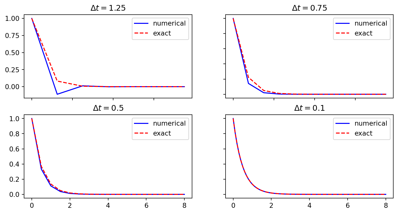
Encouraging numerical solutions - Backwards Euler
\(I=1\), \(a=2\), \(\theta =1\), \(\Delta t=1.25, 0.75, 0.5, 0.1\).

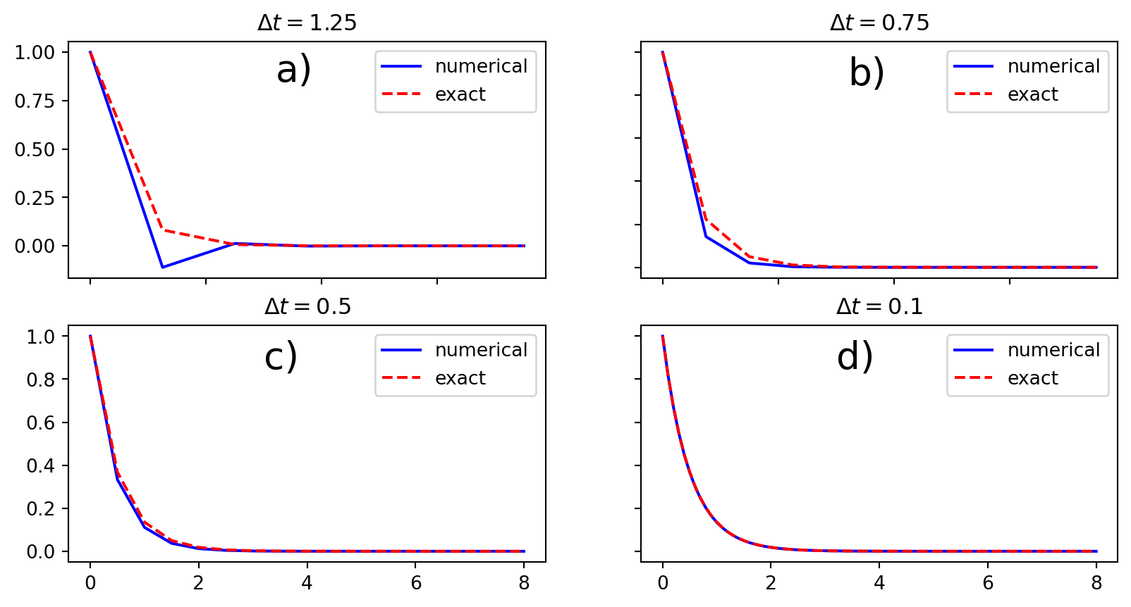
Discouraging numerical solutions - Crank-Nicolson
\(I=1\), \(a=2\), \(\theta=0.5\), \(\Delta t=1.25, 0.75, 0.5, 0.1\).
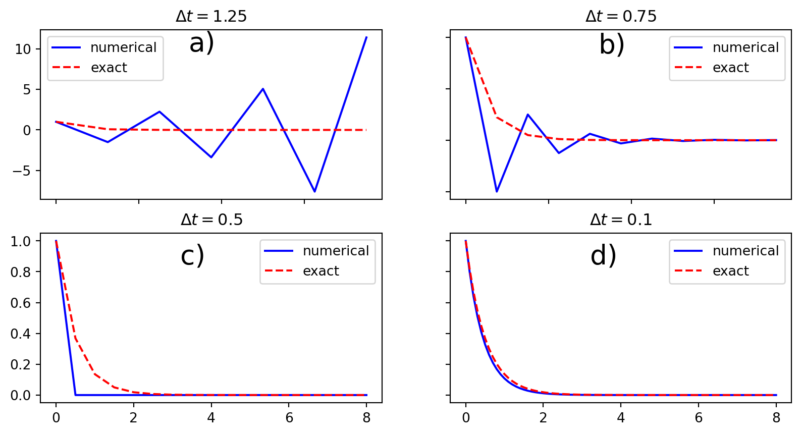
Discouraging numerical solutions - Forward Euler
\(I=1\), \(a=2\), \(\theta=0\), \(\Delta t=1.25, 0.75, 0.5, 0.1\).

Summary of observations
The characteristics of the displayed curves can be summarized as follows:
- The Backward Euler scheme always gives a monotone solution, lying above the exact solution.
- The Crank-Nicolson scheme gives the most accurate results, but for \(\Delta t=1.25\) the solution oscillates.
- The Forward Euler scheme gives a growing, oscillating solution for \(\Delta t=1.25\); a decaying, oscillating solution for \(\Delta t=0.75\); a strange solution \(u^n=0\) for \(n\geq 1\) when \(\Delta t=0.5\); and a solution seemingly as accurate as the one by the Backward Euler scheme for \(\Delta t = 0.1\), but the curve lies below the exact solution.
- Small enough \(\Delta t\) gives stable and accurate solution for all methods!
Problem setting
We ask the question
- Under what circumstances, i.e., values of the input data \(I\), \(a\), and \(\Delta t\) will the Forward Euler and Crank-Nicolson schemes result in undesired oscillatory solutions?
Techniques of investigation:
- Numerical experiments
- Mathematical analysis
Another question to be raised is
- How does \(\Delta t\) impact the error in the numerical solution?
Exact numerical solution
For the simple exponential decay problem we are lucky enough to have an exact numerical solution
\[ u^{n} = IA^n,\quad A = \frac{1 - (1-\theta) a\Delta t}{1 + \theta a\Delta t} \]
Such a formula for the exact discrete solution is unusual to obtain in practice, but very handy for our analysis here.
Note
An exact dicrete solution fulfills a discrete equation (without round-off errors), whereas an exact solution fulfills the original mathematical equation.
Stability
Since \(u^n=I A^n\),
- \(A < 0\) gives a factor \((-1)^n\) and oscillatory solutions
- \(|A|>1\) gives growing solutions
- Recall: the exact solution is monotone and decaying
- If these qualitative properties are not met, we say that the numerical solution is unstable
For stability we need
\[ A > 0 \quad \text{ and } \quad |A| \le 1 \]
Computation of stability in this problem
\(A < 0\) if
\[ \frac{1 - (1-\theta) a\Delta t}{1 + \theta a\Delta t} < 0 \]
To avoid oscillatory solutions we must have \(A> 0\), which happens for
\[ \Delta t < \frac{1}{(1-\theta)a}, \quad \text{for} \, \theta < 1 \]
- Always fulfilled for Backward Euler (\(\theta=1 \rightarrow A = 1/(1+a \Delta t) > 0\))
- \(\Delta t \leq 1/a\) for Forward Euler (\(\theta=0\))
- \(\Delta t \leq 2/a\) for Crank-Nicolson (\(\theta = 0.5\))
We get oscillatory solutions for FE when \(\Delta t \le 1/a\) and for CN when \(\Delta t \le 2/a\)
Computation of stability in this problem
\(|A|\leq 1\) means \(-1\leq A\leq 1\)
\[ -1\leq\frac{1 - (1-\theta) a\Delta t}{1 + \theta a\Delta t} \leq 1 \]
- \(-1\) is the critical limit (because \(A\le 1\) is always satisfied).
- \(-1 < A\) is always fulfilled for Backward Euler (\(\theta=1\)) and Crank-Nicolson (\(\theta=0.5\)).
- For forward Euler or simply \(\theta < 0.5\) we have \[ \Delta t \leq \frac{2}{(1-2\theta)a},\quad \] and thus \(\Delta t \leq 2/a\) for stability of the forward Euler (\(\theta=0\)) method
Explanation of problems with forward Euler
- \(a\Delta t= 2\cdot 1.25=2.5\) and \(A=-1.5\): oscillations and growth
- \(a\Delta t = 2\cdot 0.75=1.5\) and \(A=-0.5\): oscillations and decay
- \(\Delta t=0.5\) and \(A=0\): \(u^n=0\) for \(n>0\)
- Smaller \(\Delta t\): qualitatively correct solution
Explanation of problems with Crank-Nicolson
- \(\Delta t=1.25\) and \(A=-0.25\): oscillatory solution
Never any growing solution
Summary of stability
- Forward Euler is conditionally stable
- \(\Delta t < 2/a\) for avoiding growth
- \(\Delta t\leq 1/a\) for avoiding oscillations
- The Crank-Nicolson is unconditionally stable wrt growth and conditionally stable wrt oscillations
- \(\Delta t < 2/a\) for avoiding oscillations
- Backward Euler is unconditionally stable
Comparing amplification factors
\(u^{n+1}\) is an amplification \(A\) of \(u^n\):
\[ u^{n+1} = Au^n,\quad A = \frac{1 - (1-\theta) a\Delta t}{1 + \theta a\Delta t} \]
The exact solution is also an amplification:
\[ \begin{align} u(t_{n+1}) &= e^{-a(t_n+\Delta t)} \\ u(t_{n+1}) &= e^{-a \Delta t} e^{-a t_n} \\ u(t_{n+1}) &= A_e u(t_n), \quad A_e = e^{-a\Delta t} \end{align} \]
A possible measure of accuracy: \(A_e - A\)
Plotting amplification factors
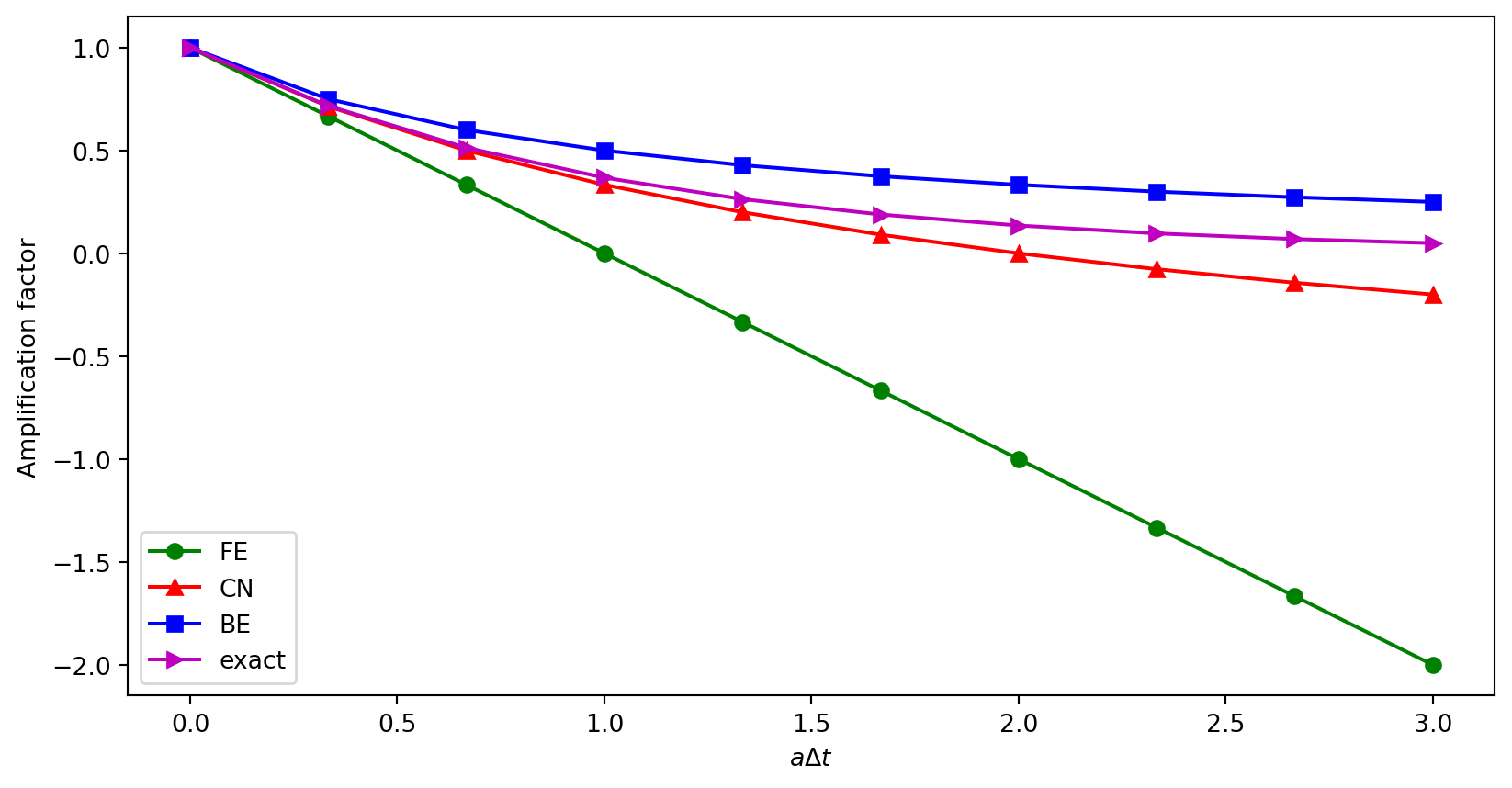
\(p=a\Delta t\) is the important parameter for numerical performance
- \(p=a\Delta t\) is a dimensionless parameter
- all expressions for stability and accuracy involve \(p\)
- Note that \(\Delta t\) alone is not so important, it is the combination with \(a\) through \(p=a\Delta t\) that matters
Another evidence why \(p=a\Delta t\) is key
If we scale the model by \(\bar t=at\), \(\bar u=u/I\), we get \(d\bar u/d\bar t = -\bar u\), \(\bar u(0)=1\) (no physical parameters!). The analysis show that \(\Delta \bar t\) is key, corresponding to \(a\Delta t\) in the unscaled model.
Series expansion of amplification factors
To investigate \(A_e - A\) mathematically, we can Taylor expand the expression, using \(p=a\Delta t\) as variable.
from sympy import *
# Create p as a mathematical symbol with name 'p'
p = Symbol('p', positive=True)
# Create a mathematical expression with p
A_e = exp(-p)
# Find the first 6 terms of the Taylor series of A_e
A_e.series(p, 0, 6)
\(\displaystyle 1 - p + \frac{p^{2}}{2} - \frac{p^{3}}{6} + \frac{p^{4}}{24} - \frac{p^{5}}{120} + O\left(p^{6}\right)\)
This is the Taylor expansion of the exact amplification factor. How does it compare with the numerical amplification factors?
Numerical amplification factors
Compute the Taylor expansions of \(A_e - A\)
from IPython.display import display
theta = Symbol('theta', positive=True)
A = (1-(1-theta)*p)/(1+theta*p)
FE = A_e.series(p, 0, 4) - A.subs(theta, 0).series(p, 0, 4)
BE = A_e.series(p, 0, 4) - A.subs(theta, 1).series(p, 0, 4)
half = Rational(1, 2)  # exact fraction 1/2
CN = A_e.series(p, 0, 4) - A.subs(theta, half).series(p, 0, 4)
display(FE)
display(BE)
display(CN)
\(\displaystyle \frac{p^{2}}{2} - \frac{p^{3}}{6} + O\left(p^{4}\right)\)
\(\displaystyle - \frac{p^{2}}{2} + \frac{5 p^{3}}{6} + O\left(p^{4}\right)\)
\(\displaystyle \frac{p^{3}}{12} + O\left(p^{4}\right)\)
- Forward/backward Euler have leading error \(p^2\), or more commonly \(\Delta t^2\)
- Crank-Nicolson has leading error \(p^3\), or \(\Delta t^3\)
The true/global error at a point
- The error in \(A\) reflects the local (amplification) error when going from one time step to the next
- What is the global (true) error at \(t_n\)?
\[ e^n = u_e(t_n) - u^n = Ie^{-at_n} - IA^n \]
- Taylor series expansions of \(e^n\) simplify the expression
Computing the global error at a point
n = Symbol('n', integer=True, positive=True)
u_e = exp(-p*n)   # I=1
u_n = A**n        # I=1
FE = u_e.series(p, 0, 4) - u_n.subs(theta, 0).series(p, 0, 4)
BE = u_e.series(p, 0, 4) - u_n.subs(theta, 1).series(p, 0, 4)
CN = u_e.series(p, 0, 4) - u_n.subs(theta, half).series(p, 0, 4)
display(simplify(FE))
display(simplify(BE))
display(simplify(CN))
\(\displaystyle \frac{n p^{2}}{2} + \frac{n p^{3}}{3} - \frac{n^{2} p^{3}}{2} + O\left(p^{4}\right)\)
\(\displaystyle - \frac{n p^{2}}{2} + \frac{n p^{3}}{3} + \frac{n^{2} p^{3}}{2} + O\left(p^{4}\right)\)
\(\displaystyle \frac{n p^{3}}{12} + O\left(p^{4}\right)\)
Substitute \(n\) by \(t/\Delta t\) and \(p\) by \(a \Delta t\):
- Forward and Backward Euler: leading order term \(\frac{1}{2} ta^2\Delta t\)
- Crank-Nicolson: leading order term \(\frac{1}{12}ta^3\Delta t^2\)
Convergence
The numerical scheme is convergent if the global error \(e^n\rightarrow 0\) as \(\Delta t\rightarrow 0\). If the error has a leading order term \((\Delta t)^r\), the convergence rate is of order \(r\).
Integrated errors
The \(\ell^2\) norm of the numerical error is computed as
\[ ||e^n||_{\ell^2} = \sqrt{\Delta t\sum_{n=0}^{N_t} ({u_{e}}(t_n) - u^n)^2} \]
We can compute this using Sympy. Forward/Backward Euler has \(e^n \sim np^2/2\)
h, N, a, T = symbols('h,N,a,T') # h represents Delta t
simplify(sqrt(h * summation((n*p**2/2)**2, (n, 0, N))).subs(p, a*h).subs(N, T/h))
\(\displaystyle \frac{\sqrt{6} a^{2} h^{2} \sqrt{T \left(\frac{2 T^{2}}{h^{2}} + \frac{3 T}{h} + 1\right)}}{12}\)
If we keep only the leading term in the parenthesis, we get the first order \[ ||e^n||_{\ell^2} \approx \frac{1}{2}\sqrt{\frac{T^3}{3}} a^2\Delta t \]
Crank-Nicolson
For Crank-Nicolson the pointwise error is \(e^n \sim n p^3 / 12\). We get
\(\displaystyle \frac{\sqrt{6} a^{3} h^{3} \sqrt{T \left(\frac{2 T^{2}}{h^{2}} + \frac{3 T}{h} + 1\right)}}{72}\)
which is simplified to the second order accurate
\[ ||e^n||_{\ell^2} \approx \frac{1}{12}\sqrt{\frac{T^3}{3}}a^3\Delta t^2 \]
Summary of errors
Analysis of both the pointwise and the time-integrated true errors:
- 1st order for Forward and Backward Euler
- 2nd order for Crank-Nicolson
Truncation error
- How good is the discrete equation?
- Possible answer: see how well \(u_{e}\) fits the discrete equation
Consider the forward difference equation \[ \frac{u^{n+1}-u^n}{\Delta t} = -au^n \]
Insert \(u_{e}\) to obtain a truncation error \(R^n\)
\[ \frac{u_{e}(t_{n+1})-u_{e}(t_n)}{\Delta t} + au_{e}(t_n) = R^n \neq 0 \]
Computation of the truncation error
- The residual \(R^n\) is the truncation error. How does \(R^n\) vary with \(\Delta t\)?
Tool: Taylor expand \(u_{e}\) around the point where the ODE is sampled (here \(t_n\))
\[ u_{e}(t_{n+1}) = u_{e}(t_n) + u_{e}'(t_n)\Delta t + \frac{1}{2}u_{e}''(t_n) \Delta t^2 + \cdots \]
Inserting this Taylor series for \(u_{e}\) in the forward difference equation
\[ R^n = \frac{u_{e}(t_{n+1})-u_{e}(t_n)}{\Delta t} + au_{e}(t_n) \]
to get
\[ R^n = u_{e}'(t_n) + \frac{1}{2}u_{e}''(t_n)\Delta t + \ldots + au_{e}(t_n) \]
The truncation error forward Euler
We have \[ R^n = u_{e}'(t_n) + \frac{1}{2}u_{e}''(t_n)\Delta t + \ldots + au_{e}(t_n) \]
Since \(u_{e}\) solves the ODE \(u_{e}'(t_n)=-au_{e}(t_n)\), we get that \(u_{e}'(t_n)\) and \(au_{e}(t_n)\) cancel out. We are left with leading term
\[ R^n \approx \frac{1}{2}u_{e}''(t_n)\Delta t \]
This is a mathematical expression for the truncation error.
The truncation error for other schemes
Backward Euler:
\[ R^n \approx -\frac{1}{2}u_{e}''(t_n)\Delta t \]
Crank-Nicolson:
\[ R^{n+\scriptstyle\frac{1}{2}} \approx \frac{1}{24}u_{e}'''(t_{n+\scriptstyle\frac{1}{2}})\Delta t^2 \]
Consistency, stability, and convergence
Truncation error measures the residual in the difference equations. The scheme is consistent if the truncation error goes to 0 as \(\Delta t\rightarrow 0\). Importance: the difference equations approaches the differential equation as \(\Delta t\rightarrow 0\).
Stability means that the numerical solution exhibits the same qualitative properties as the exact solution. Here: monotone, decaying function.
Convergence implies that the true (global) error \(e^n =u_{e}(t_n)-u^n\rightarrow 0\) as \(\Delta t\rightarrow 0\). This is really what we want!
The Lax equivalence theorem for linear differential equations: consistency + stability is equivalent with convergence.
(Consistency and stability is in most problems much easier to establish than convergence.)
Numerical computation of convergence rate
We assume that the \(\ell^2\) error norm on the mesh with level \(i\) can be written as
\[ E_i = C (\Delta t_i)^r \]
where \(C\) is a constant. This way, if we have the error on two levels, then we can compute
\[ \frac{E_{i-1}}{E_i} = \frac{ (\Delta t_{i-1})^r}{(\Delta t_{i})^r} = \left( \frac{\Delta t_{i-1}}{ \Delta t_i} \right)^r \]
and isolate \(r\) by computing
\[ r = \frac{\log {\frac{E_{i-1}}{E_i}}}{\log {\frac{\Delta t_{i-1}}{\Delta t_i}}} \]
Function for convergence rate
u_exact = lambda t, I, a: I*np.exp(-a*t)

def l2_error(I, a, theta, dt):
    u, t = solver(I, a, T, dt, theta)
    en = u_exact(t, I, a) - u
    return np.sqrt(dt*np.sum(en**2))

def convergence_rates(m, I=1, a=2, T=8, theta=1, dt=1.):
    dt_values, E_values = [], []
    for i in range(m):
        E = l2_error(I, a, theta, dt)
        dt_values.append(dt)
        E_values.append(E)
        dt = dt/2
    # Compute m-1 orders that should all be the same
    r = [np.log(E_values[i-1]/E_values[i])/
         np.log(dt_values[i-1]/dt_values[i])
         for i in range(1, m, 1)]
    return r
Test convergence rates
Backward Euler:
[np.float64(0.9619265651066382),
 np.float64(0.98003334385805),
 np.float64(0.9897576131285538)]
Forward Euler:
[np.float64(1.0472640894307232),
 np.float64(1.0222599097461846),
 np.float64(1.0108154242259877)]
Crank-Nicolson:
[np.float64(2.0037335266421343),
 np.float64(2.0009433957768175),
 np.float64(2.000236481071457)]
All in good agreement with theory:-)