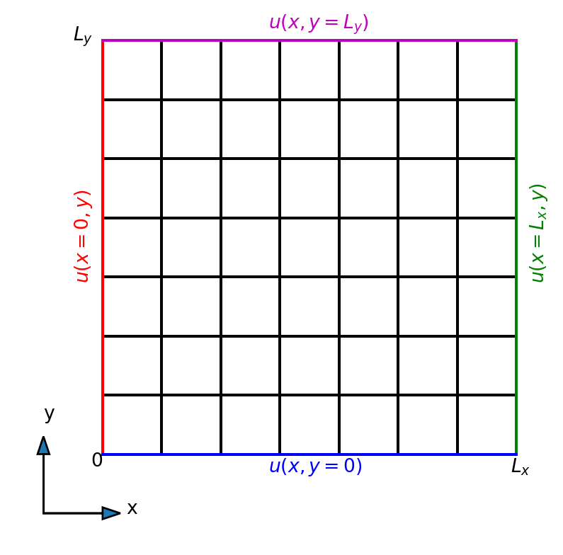
Boundary conditions on any side may be a function of the non-constant variable \[\begin{align*}
\color{red}{ u(x=0, y)} &= f(y) \\
\color{blue}{u(x, y=0)} &= f(x)
\end{align*}\]
where \(f\) is a function of one variable, \(f: \mathbb{R}\rightarrow \mathbb{R}\)
Note
The boundary conditions need to be consistent in the corners, because each corner belongs to two sides.
Discretization
We discretize the mesh using two lines, one in the \(x\)-direction and one in the \(y\)-direction:
\[
x_i = i \Delta x, \quad i = 0, 1, \ldots, N_x
\]
The outcome is a tuple containing all possible ordered pairs of items, where the first item is from \(\boldsymbol{u}\) and the second from \(\boldsymbol{v}\).
Note
Tuples are immutable sequences.
Mathematical description of the Cartesian product
The Cartesian product can be described mathematically as
\[
\boldsymbol{u} \times \boldsymbol{v} = \{ (u, v) \, | \, u \in \boldsymbol{u} \text{ and } v \in \boldsymbol{v} \},
\]
which reads the set of all pairs \((u, v)\) such that \(u\) is in the set \(\boldsymbol{u}\) and \(v\) in the set \(\boldsymbol{v}\).
Note
Sets are unordered collections with no duplicate elements.
Sets are written with curly brackets.
The pairs \((u, v)\) are not sets since the order of the numbers is important.
itertools work on any kind of sequence.
Why is this relevant for computational meshes?
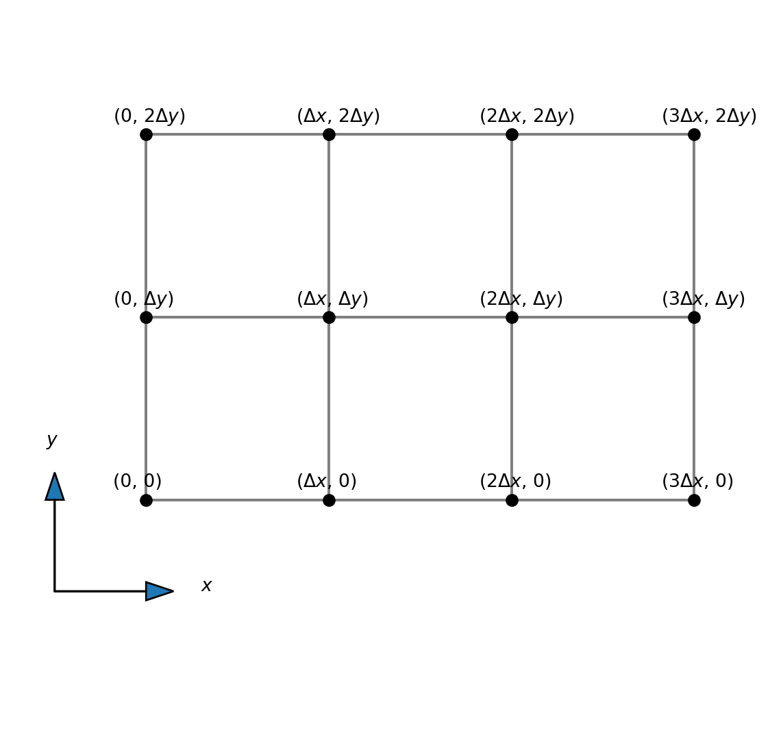
Structured 2D meshes
We have grid lines \[
\boldsymbol{x} = (x_0, x_1, \ldots, x_{N_x}) = (0, \Delta x, 2 \Delta x, \ldots, L_x)
\]\[
\boldsymbol{y} = (y_0, y_1, \ldots, y_{N_y}) = (0, \Delta y, 2 \Delta y, \ldots, L_y)
\]
The computational mesh is a Cartesian product!
The mesh is all pairs \((x, y)\) such that \(x\) is in \(\boldsymbol{x}\) and \(y\) is in \(\boldsymbol{y}\).
\[
\boldsymbol{x} \times \boldsymbol{y} = \{(x, y) \, | \, x \in \boldsymbol{x} \text{ and } y \in \boldsymbol{y} \}
\]
However, the numbers are naturally seen as points in a 2D mesh:
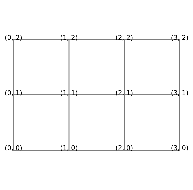
A complicating factor for the mesh
Note
If this mesh was a 2D matrix, then \(i\) and \(j\) in \((i, j)\) would represent column and row, respectively, which is counterintuitive.
We normally think about a matrix \(A\) with items \(a_{ij}\), where the first index \(i\) represents row and second \(j\) represents column.
This is a complicating factor for the Cartesian mesh that is important to be aware of. But it is not a mistake. The numbers in the plot above are not indices of a matrix, they represent \((x, y)\) in a Cartesian mesh!
Numpy meshgrid
Let us now compute our Cartesian mesh using numpy.meshgrid. We have the 1D mesh arrays
The added dimension of length 1 is important for how the array broadcasts. The extra dimension tells Numpy that the array is constant along this other axis. That is, mesh[0] is constant along the second axis, no matter what size the second axis is. Similarly, mesh[1] is constant along the first axis. And since the 2D array is constant along that direction it is not necessary to actually store the numbers! So this is memory efficient.
So what happens if you now have this sparse mesh and you create a mesh function
\[
f(x, y) = x + y
\]
Broadcasting 2
Compute \[
f(x, y) = x + y
\]
when \(x\) and \(y\) are stored using sparse matrices of shape \((4, 1)\) and \((1, 3)\)
The shape of \(f\) is \((4, 3)\)! Exactly as it would be without the sparse matrices!
Two-dimensional mesh function
A mesh function on the two-dimensional domain will now be denoted as
\[
u_{ij} = u(x_i, y_j).
\]
The mesh function is a dense two-dimensional array of shape \({(N_x+1)\times (N_y+1)}\) and we will write \(U = (u_{ij})_{i,j=0}^{N_x, N_y}\). It may also be considered a matrix.
For the component \(u_{ij}\), we note that \(i\) represents row and \(j\) represents column. This is matrix storage, like we got for meshgrid using indexing="ij".
Row-major computer storage
In Python a matrix is row-major. This means that the matrix that looks like
The computer does not know anything about these numbers belonging to a two-dimensional array. The computer only knows that \((N_x+1)(N_y+1)\) numbers are stored side by side.
More on row-major storage
We can get the single row \(i\) of the \(U\) matrix as \(u_i = (u_{i,0}, u_{i,1}, \ldots, u_{i, N_y})\). For example,
U = np.arange(9).reshape((3, 3))display(U)display(U[0])display(U[1])display(U[2])
How to compute \(\frac{\partial^2 u}{\partial x^2}\)?
Use the one-dimensional derivative matrix \(D^{(2)}\) along the first axis of \(U=(u_{i,j})_{i,j=0}^{N_x, N_y}\)
\[
D^{(2)} U = \sum_{k=0}^{N_x} d^{(2)}_{ik} u_{k,j}
\]
So \(D^{(2)} U\) is a matrix-matrix product between the two matrices \(D^{(2)}\in \mathbb{R}^{(N_x+1)\times (N_x+1)}\) and \(U \in \mathbb{R}^{(N_x+1) \times (N_y+1)}\), such that \(D^{(2)}U \in \mathbb{R}^{(N_x+1) \times (N_y+1)}\)
Using now that \(\partial^2 u/\partial x^2 = D_x^{(2)}U\) and \(\partial^2 u/\partial y^2 = U(D_y^{(2)})^T\) we can write Poisson’s equation on discretized (and matrix) form as
\[
D_x^{(2)} U + U (D_y^{(2)})^T = F,
\]
where the mesh function \(F = (f(x_i, y_j))_{i,j=0}^{N_x, N_y}\).
How can we solve this equation for the unknown matrix \(U\)?
Can we write this equation as
\[
Ax = b
\]
where \(A\) is the coefficient matrix, \(x\) is the unknown vector and \(b\) is the rhs vector?
Can we transform our unknown matrix \(U\) into a vector?
Vectorization (the vec-trick)
Consider first for simplicity a \(2 \times 2\) matrix
\[
A =
\begin{bmatrix}
a & b \\
c & d
\end{bmatrix}
\]
In general, a row-major vectorization transforms the matrix into a vector as follows
\[
\begin{bmatrix}
a & b \\
c & d
\end{bmatrix}
\longrightarrow
\begin{bmatrix}
a & b & c & d
\end{bmatrix}^T =
\begin{bmatrix}
a \\
b \\
c \\
d
\end{bmatrix}
\]
This operation is referred to as vec(A) and thus
\[
\text{vec}(A) = \begin{bmatrix}
a & b & c & d
\end{bmatrix}^T
\]
Note
The vec-trick transforms a matrix into a vector! Just like numpy.ravel.
Just check that this corresponds to \[
\begin{align*}
c_{00} &= a_{00}b_{00} + a_{01}b_{10} \\
c_{01} &= a_{00}b_{01} + a_{01}b_{11} \\
c_{10} &= a_{10}b_{00} + a_{11}b_{10} \\
c_{11} &= a_{10}b_{01} + a_{11}b_{11}
\end{align*}
\]
The Kronecker product
If \(A\) and \(B\) are matrices of dimensions \(p \times q\) and \(r \times s\), respectively, then \(A \otimes B\) is the matrix of dimension \(pr \times qs\), with \(p \times q\) block form, where the \(i, j\) block is \(a_{ij}B\). The Kronecker product is most simply illustrated for two small matrices of shape \(2 \times 2\):
\[
\begin{bmatrix}
1 & 2 \\
3 & 4
\end{bmatrix}
\otimes
\begin{bmatrix}
a & b \\
c & d
\end{bmatrix}
=
\left(\begin{array}{c|c}
\begin{matrix}
a & b \\
c & d
\end{matrix}
& \begin{matrix}
2a & 2b \\
2c & 2d
\end{matrix} \\
\hline
\begin{matrix}
3a & 3b \\
3c & 3d
\end{matrix} &
\begin{matrix}
4a & 4b \\
4c & 4d
\end{matrix}
\end{array}\right)
\]
For diagonal matrices it is simpler
\[
\begin{bmatrix}
1 & 0 \\
0 & 1
\end{bmatrix}
\otimes
\begin{bmatrix}
a & b \\
c & d
\end{bmatrix}
=
\left(\begin{array}{c|c}
\begin{matrix}
a & b \\
c & d
\end{matrix}
&
\begin{matrix}
0 & 0 \\
0 & 0
\end{matrix}
\\
\hline
\begin{matrix}
0 & 0 \\
0 & 0
\end{matrix} &
\begin{matrix}
a & b \\
c & d
\end{matrix}
\end{array}\right)
\]
and
\[
\begin{bmatrix}
a & b \\
c & d
\end{bmatrix}
\otimes
\begin{bmatrix}
1 & 0 \\
0 & 1
\end{bmatrix}
=
\left(\begin{array}{c|c}
\begin{matrix}
a & 0 \\
0 & a
\end{matrix}
& \begin{matrix}
b & 0 \\
0 & b
\end{matrix} \\
\hline
\begin{matrix}
c & 0 \\
0 & c
\end{matrix} &
\begin{matrix}
d & 0 \\
0 & d
\end{matrix}
\end{array}\right)
\]
The vec-trick for matrix products
A very useful result is
\[
\text{vec}(ABC^T) = (A \otimes C) \text{vec}(B)
\]
Hence in the example from before with \(C=AB\):
\[\text{vec}(C) = \text{vec}(AB) = \text{vec}(ABI) = (A \otimes I) \text{vec}(B)\]
\[
A \otimes I =
\begin{bmatrix}
a_{00} & 0 & a_{01} & 0 \\
0 & a_{00} & 0 & a_{01} \\
a_{10} & 0 & a_{11} & 0 \\
0 & a_{10} & 0 & a_{11} \\
\end{bmatrix}
\] where \(I\) is the identity matrix.
The vec-trick for derivatives in 2D
Consider the second derivative in the \(x\)-direction
This is a linear equations of type \(Ax=b\), where \(A = D_x^{(2)} \otimes I_{y} + I_{x} \otimes D_y^{(2)}\), \(x = \text{vec}(U)\) and \(b = \text{vec}(F)\).
Note
Vectorization is a linear process that allows us to transform a matrix into a vector. Through vectorization we can express matrix-multiplication through a larger matrix using the Kronecker product.
The Laplace operator
The Laplace operator \(\nabla^2\) applied to a two-dimensional field \(u(x, y)\) in Cartesian coordinates is
But where are all the boundary points? Can we manipulate the matrix \(M\) in order to fix Dirichlet boundary conditions?
We can do this by identing all rows of M corresponding to a boundary point. But which indices in M correspond to boundaries? We can find this easily with a little slicing and trickery. Lets create a mesh function B that is one on the boundary and zero elsewhere
U = sparse.linalg.spsolve(A, b)U = np.reshape(U, (Nx+1, Ny+1))plt.contourf(xij, yij, U, 100);
Summary
Two-dimensional problems on simple Cartesian domains make use of Cartesian products to create structured uniform meshes.
In 2D the unknown meshfunction \(U=(u_{ij})_{i,j=0}^{N_x,N_y}\) is a matrix and not a vector.
In order to use regular linear algebra solvers and recast the problem as \[Ax=b\] we make use of the veck-trick and the Kronecker product
The vec-trick transforms a matrix into a vector \[
A = \begin{bmatrix}
a & b \\ c & d
\end{bmatrix} \quad \rightarrow \quad
\text{vec}(A) = \begin{bmatrix}
a & b & c & d
\end{bmatrix}^T
\]
The vec-trick transforms matrix-matrix products using the Kronecker product \[\text{vec}(ABC^T) = (A \otimes C) \text{vec}(B)\]
Summary continued
The Poisson equation in 2D reads \[
D_x^{(2)} U + U (D_y^{(2)})^T = F
\]
Regular linear algebra cannot easily solve the above since the unknown is a matrix. Hence we transform the equation using the vec-trick \[
\underbrace{\left(D_x^{(2)} \otimes I_{y} + I_{x} \otimes D_y^{(2)} \right)}_{M} \text{vec}(U) = \text{vec}(F)
\]
and solve \[
\text{vec}(U) = M^{-1} \text{vec}(F)
\]