Solving PDEs with the method of weighted residuals
MATMEK-4270
Prof. Mikael Mortensen, University of Oslo
Recap
We have until now considered the approximation of a function \(u(x)\) using a function space \(V_N = \text{span}\{\psi_j\}_{j=0}^N\)
\[
u_N(x) \approx u(x), \quad u_N(x) = \sum_{j=0}^N \hat{u}_j \psi_j(x)
\]
In order to find the unknowns (degrees of freedom) \(\{\hat{u}_j\}_{j=0}^N\) we have considered the error \(e=u_N-u\) through various methods
Variational methods
Collocation
We will now learn to approximate \(\small u(x)\) by \(\small u_N(x)\) such that it satisfies a linear equation
\[
\mathcal{L}(u) = f
\]
where the generic operator \(\mathcal{L}(u)\) can represent anything, like
\[
\begin{align*}
u &= f \\
u' &= f \\
u'' &= f \\
u'' +\alpha u' + \lambda u &= f \\
\frac{d}{dx}\left(\alpha \frac{d u}{dx}\right) &= f
\end{align*}
\]
Function approximation is then simply the case \(u=f\) , such that \(u_N \approx f\) .
Define a new error measure (the residual) that we ultimately want to be zero
\[
\mathcal{R} = \mathcal{L}(u)-f
\]
and create a “numerical” residual by inserting for \(u = u_N\)
\[
\mathcal{R}_N = \mathcal{L}(u_N)-f
\]
The task now is to minmize \(\mathcal{R}_N\) in order to find the unknowns that are still \(\{\hat{u}_j\}_{j=0}^N\) .
For function approximation \(\mathcal{R}_N = e = u_N - f = u_N - u\) .
The method of weighted residuals (MWR)
is defined such that the residual (with \(u_N \in V_N\) ) must satisfy
\[
(\mathcal{R}_N, v) = 0 \quad \forall \, v \in W
\]
for some (possibly different) functionspace \(W\) .
This is a generic method, where the choice of \(V_N\) and \(W\) fully determines the method.
Note the similarity to function approximation
\[
(u_N - u, v) = (e, v) = 0
\]
Now we have instead the slightly more complicated
\[
(\mathcal{L}(u_N)-f, v) = (\mathcal{R}_N, v) = 0
\]
The Galerkin method is a MWR with \(W=V_N\)
Find \(u_N \in V_N\) such that
\[
(\mathcal{R}_N, v)=(\mathcal{L}(u_N)-f, v)=0, \quad \forall \, v \in V_N
\]
The residual (or error) is orthogonal to all the test functions. We can also write this as
\[
(\mathcal{L}(u_N)-f, \psi_j)=0, \quad j=0,1,\ldots, N
\]
The least squares method is a MWR with \(\small W=\text{span}\{\frac{\partial \mathcal{R}_N}{\partial \hat{u}_j}\}_{j=0}^N\)
since \[
\frac{\partial (\mathcal{R_N}, \mathcal{R}_N)}{\partial \hat{u}_j} = 0, \quad j = 0, 1, \ldots, N
\]
can be written as
\[
\left(\mathcal{R}_N, \frac{\partial \mathcal{R}_N}{\partial \hat{u}_j}\right)=0, \quad j = 0, 1, \ldots, N
\]
The collocation method is to find
\[
\mathcal{R}_N(x_j) = 0, \quad j = 0, 1, \ldots, N
\]
for some chosen mesh points \(\{x_j\}_{j=0}^N\) .
If we write the inner products \((\mathcal{R}_N, v)\) as
\[
(\mathcal{R}_N, \psi_j) = 0, \quad j=0, 1, \ldots, N
\]
and use Dirac’s delta function as test functions \(\psi_j = \delta(x-x_j)\) , then
\[
(\mathcal{R}_N, \psi_j) = \int_{\Omega} \mathcal{R}_N(x) \delta(x-x_j) dx = \mathcal{R}_N(x_j)
\]
So the collocation method can technically also be considered a MWR!
However, collocation is not a regular variational method since \(\delta(x)\) is a distribution and
\[W \ne \text{span}\{\delta(x-x_i)\}_{i=0}^N\]
The MWR is thus
Find \(u_N \in V_N\) such that
\[
(\mathcal{R}_N, v) = 0, \quad \forall v \in W
\]
\(N+1\) equations for \(N+1\) unknowns!
Find \(\{\hat{u}_j\}_{j=0}^N\) by choosing \(N+1\) test functions for \(W\) . Choose test functions (basis functions for \(W\) ) using either one of:
Galerkin
Least squares
Collocation
First example - Poisson’s equation
\[
\begin{align}
u''(x) &= f(x), \quad x \in (-1, 1) \\
u(-1) &= u(1) = 0
\end{align}
\]
Find \(u_N \in V_N\) such that
\[
(u_N''-f, v) = 0, \quad \forall \, v \in W
\]
How to choose \(V_N\) and \(W\) ? How do we satisfy the 2 boundary conditions?
If we choose all the trial functions \(\psi_j\) such that
\[
\psi_j(\pm 1) = 0
\]
then, regardless the values of \(\{\hat{u}_j\}_{j=0}^N\)
\[
u_N(\pm 1) = \sum_{j=0}^N \hat{u}_j \psi_j(\pm 1) = 0
\]
First choice for trial functions in \(V_N\)
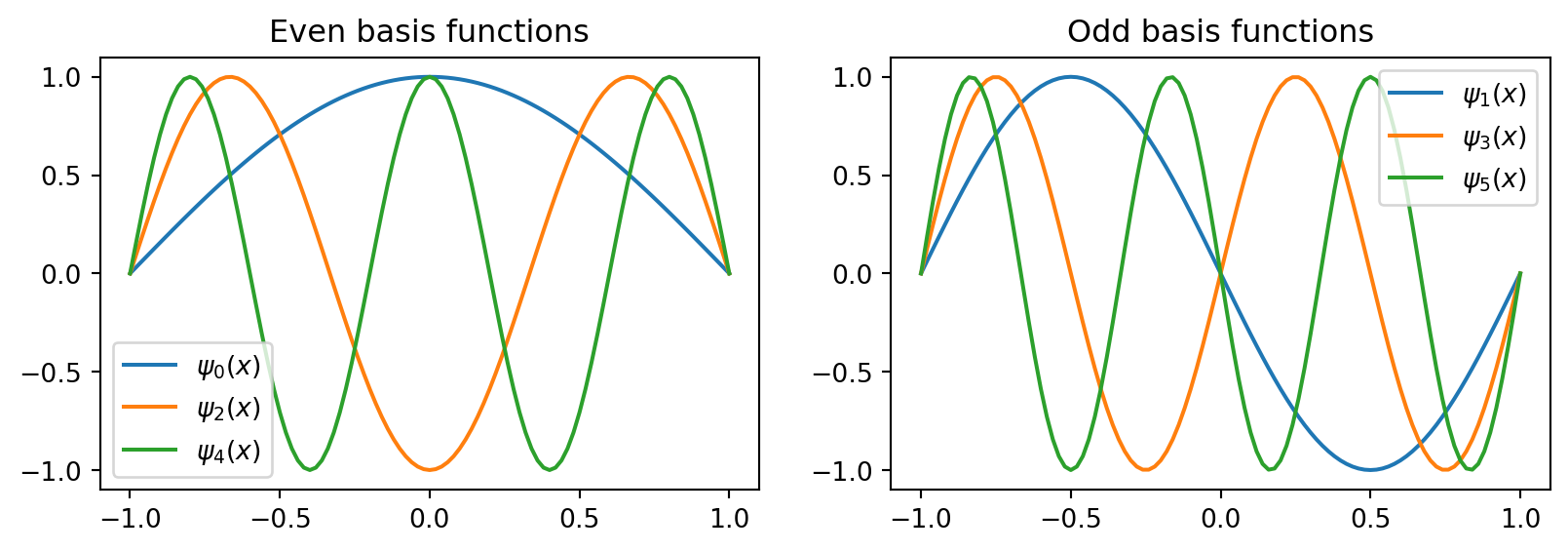
The domain is \([-1, 1]\) , so a sensible choice for \(j\ge 0\) is
\[
\psi_j(x) = \sin(\pi (j+1) (x+1)/2)
\]
The \((j+1)\) is there because we start at \(j=0\) and \(\sin(0)=0\) is not a basis function. These sines are also alternating odd/even functions.
In comparison the (unmapped) sine functions \(\sin(\pi(j+1)x), x \in [-1, 1]\) are odd for all integer \(j \ge 0\)
Solve Poisson’s equation
Insert for \(u_N=\sum_{j=0}^N \hat{u}_j \psi_j\) and \(v=\psi_i\) and obtain the linear algebra problem
\[
\sum_{j=0}^N \left(\psi''_j, \psi_i \right) \hat{u}_j = (f, \psi_i), \quad i = 0, 1, \ldots, N
\]
Consider using integration by parts
\[
\int_{a}^b u' v dx = -\int_a^b u v' dx + [u v]_{a}^b
\]
Set \(u=u'\) to obtain
\[
\int_{a}^b u'' v dx = -\int_a^b u' v' dx + [u' v]_{a}^b
\]
\[
\longrightarrow \left(\psi''_j, \psi_i \right) = -\left( \psi'_j, \psi'_i \right) + [\psi'_j \psi_i]_{-1}^1
\]
Poisson’s equation with integration by parts
Since \(\psi_j(\pm 1) = 0\) for all \(j\ge 0\) we get that
\[
\left(\psi''_j, \psi_i \right) = -\left( \psi'_j, \psi'_i \right) + \cancel{[\psi'_j \psi_i]_{-1}^1}
\]
Hence Poisson’s equation gets two alternative forms
\[
\sum_{j=0}^N \left(\psi''_j, \psi_i \right) \hat{u}_j = (f, \psi_i), \quad i = 0, 1, \ldots, N \tag{1}
\]
\[
\sum_{j=0}^N \left(\psi'_j, \psi'_i \right) \hat{u}_j = -(f, \psi_i), \quad i = 0, 1, \ldots, N \tag{2}
\]
The integration by parts is not really necessary here, as it is actually just as easy to compute \(\left(\psi''_j, \psi_i \right)\) as \(\left(\psi'_j, \psi'_i \right)\) !
Find the stiffness matrix \((\psi''_j, \psi_i)\)
\[
\begin{align*}
(\psi''_j, \psi_i) &= \Big((\sin( \pi (j+1) (x+1)/2))'', \, \sin(\pi (i+1)(x+1)/2) \Big) \\
&= -\frac{(j+1)^2\pi^2}{4} \Big(\sin(\pi (j+1)(x+1)/2), \, \sin(\pi (i+1) (x+1)/2) \Big) \\
&= -\frac{(j+1)^2 \pi^2}{4} \delta_{ij}
\end{align*}
\]
Solve problem
\[
\sum_{j=0}^N \left(\psi''_j, \psi_i \right) \hat{u}_j = (f, \psi_i), \quad i = 0, 1, \ldots, N
\]
\[
\longrightarrow \hat{u}_i = \frac{-4}{(i+1)^2 \pi^2}\Big(f,\, \sin( \pi (i+1)(x+1)/2)\Big), \quad i = 0, 1, \ldots, N
\]
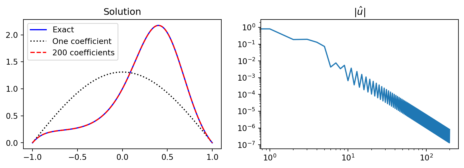
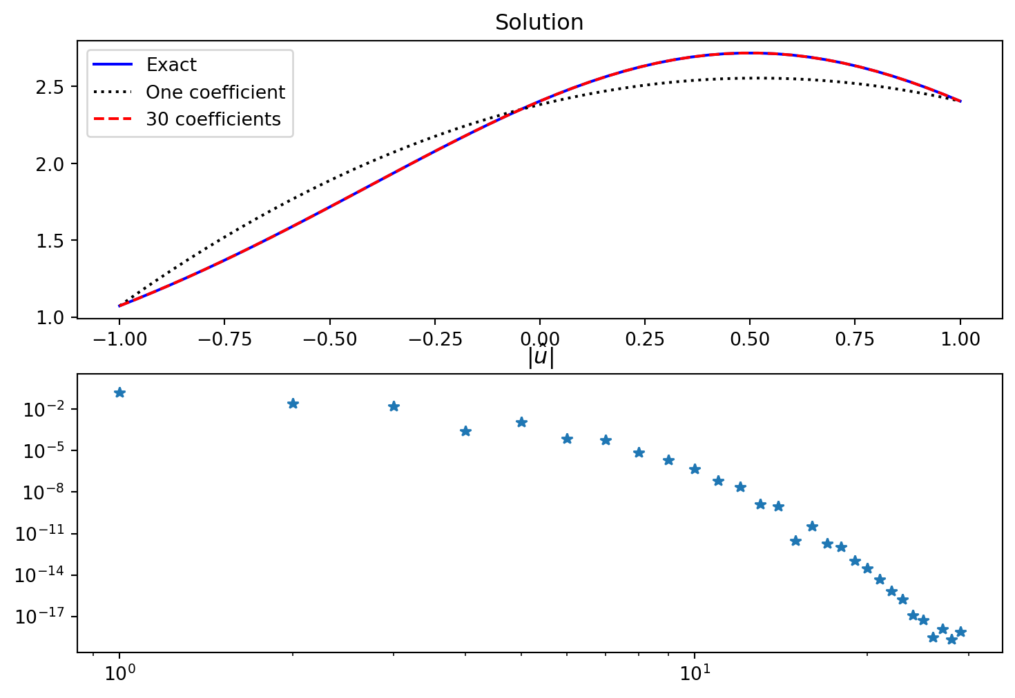
Implementation using the method of manufactured solution
from scipy.integrate import quad= sp.Symbol('x' )= (1 - x** 2 )* sp.exp(sp.cos(sp.pi* (x- 0.5 )))= ue.diff(x, 2 ) # manufactured f=u'' = lambda j: - (4 / (j+ 1 )** 2 / np.pi** 2 )* quad(sp.lambdify(x, f* sp.sin((j+ 1 )* sp.pi* (x+ 1 )/ 2 )), - 1 , 1 )[0 ]= [uhat(k) for k in range (200 )]= np.linspace(- 1 , 1 , 201 )= np.sin(np.pi/ 2 * (np.arange(len (uh))[None , :]+ 1 )* (xj[:, None ]+ 1 ))= plt.subplots(1 , 2 , figsize= (10 , 3 ))= sp.lambdify(x, ue)(xj)'b' , xj, sines[:, :1 ] @ np.array(uh)[:1 ], 'k:' ,@ np.array(uh), 'r--' )abs (np.array(uh)))'Exact' , 'One coefficient' , f' { 200 } coefficients' ])'Solution' ); ax2.set_title(r' $ | \ hat{u} | $ ' );
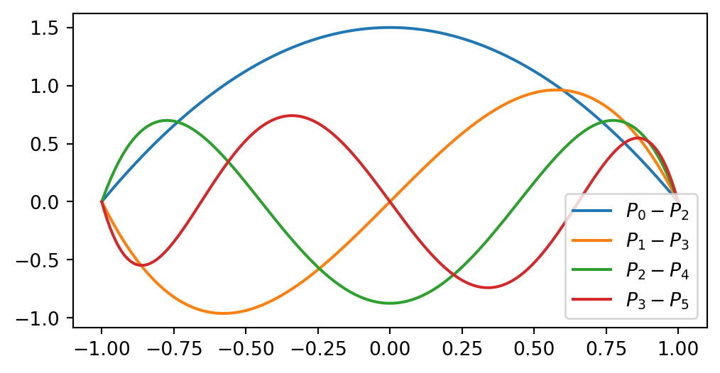
Another alternating odd/even basis can be created from Legendre polynomials \(P_j(x)\)
\[
\begin{align}
\psi_j(x) &= P_j(x) - P_{j+2}(x)\\
\psi_j(\pm 1) &= 0
\end{align}
\]
Remember that
\[
P_j(-1) = (-1)^j \quad \text{and} \quad P_j(1) = 1.
\]
Hence for any \(j\) all basis functions are zero
\[
\begin{align}
P_j(-1) - P_{j+2}(-1) &= (-1)^j - (-1)^{j+2} = 0 \\
P_j(1)-P_{j+2}(1) & =1-1=0
\end{align}
\]
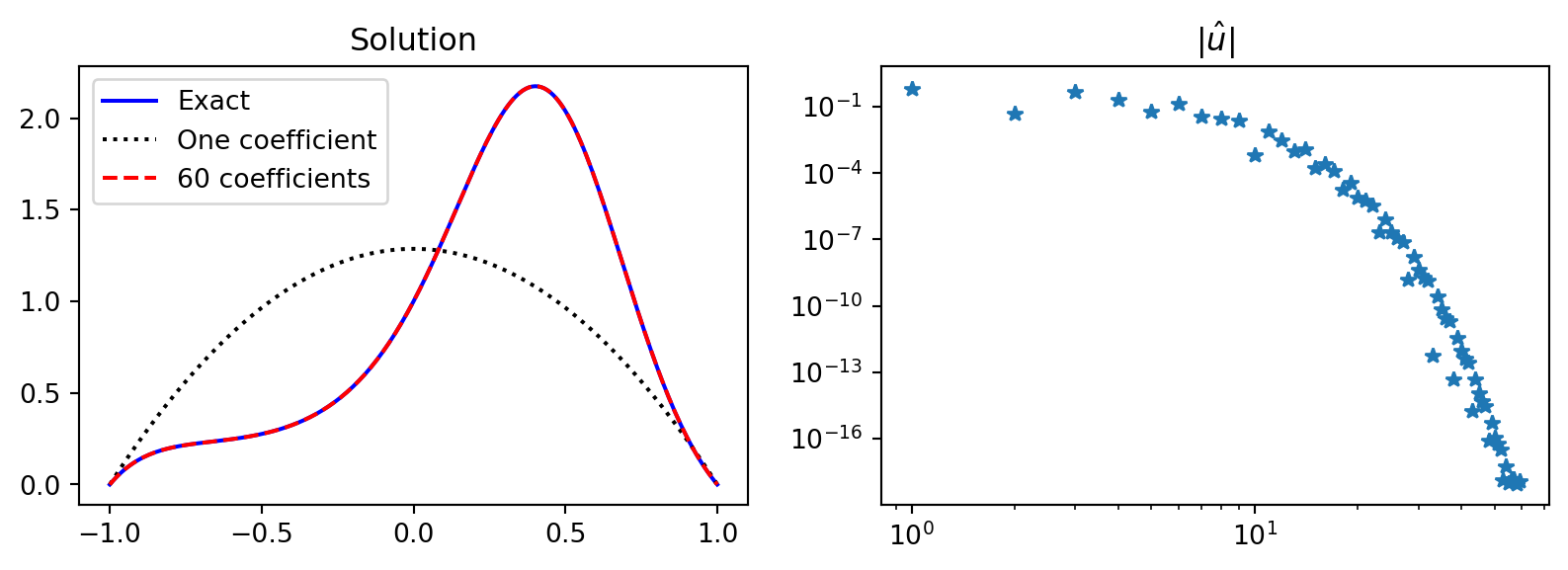
Solve Poisson’s equation with composite Legendre basis
The Legendre polynomials come with a lot of formulas, where two are \[
(P_j, P_i) = \frac{2}{2i+1}\delta_{ij} \quad \text{and} \quad (2i+3)P_{i+1} = P'_{i+2}-P'_{i}
\]
The second is very useful for computing the diagonal (!) stiffness matrix
\[
\begin{align}
(\psi'_j, \psi'_i) &= (P'_j-P'_{j+2}, P'_i-P'_{i+2}) \\
&= (-(2j+3) P_{j+1}, -(2i+3)P_{i+1}) \\
&= (2i+3)^2 (P_{j+1}, P_{i+1}) \\
&= (2i+3)^2 \frac{2}{2(i+1)+1} \delta_{i+1,j+1} \\
&= (4i+6)\delta_{ij}
\end{align}
\]
\[
\text{Solve Poisson's equation: } \longrightarrow \hat{u}_i = \frac{-\left(f, \psi_i\right)}{4i+6}
\]
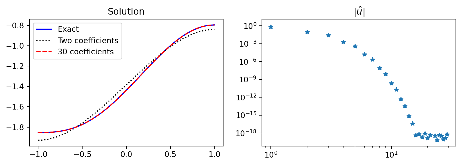
Implementation
from numpy.polynomial import Legendre as Leg= lambda j: Leg.basis(j)- Leg.basis(j+ 2 )= sp.lambdify(x, f)def uv(xj, j): return psi(j)(xj) * fl(xj)= lambda j: (- 1 / (4 * j+ 6 ))* quad(uv, - 1 , 1 , args= (j,))[0 ]= 60 = [uhat(j) for j in range (N)]= sp.Symbol('j' , integer= True , positive= True )= np.polynomial.legendre.legvander(xj, N+ 1 )= V[:, :- 2 ] - V[:, 2 :]= plt.subplots(1 , 2 , figsize= (10 , 3 ))'b' ,1 ] @ np.array(uL)[:1 ], 'k:' ,@ np.array(uL), 'r--' )abs (np.array(uL)), '*' )'Exact' , 'One coefficient' , f' { N} coefficients' ])'Solution' )r' $ | \ hat{u} | $ ' );
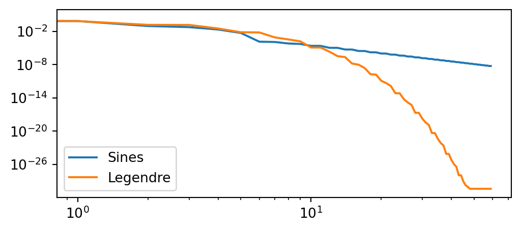
\(L^2(\Omega)\) error for sines and Legendre\[
L^2(\Omega) = \sqrt{\int_{-1}^1(u-u_e)^2dx}
\]
= np.array(uh)= np.array(uL)= np.zeros((2 , N))for n in range (N):= sines[:, :n] @ uh[:n]= Ps[:, :n] @ uL[:n]0 , n] = np.trapz((us- uej)** 2 , dx= (xj[1 ]- xj[0 ]))1 , n] = np.trapz((ul- uej)** 2 , dx= (xj[1 ]- xj[0 ]))= (6 , 2.5 ))'Sines' , 'Legendre' ])
Why are the Legendre basis functions better than the sines?
All the sine basis functions \(\psi_j=\sin(\pi(j+1)(x+1)/2)\) have even derivatives equal to zero at the boundaries, unlike the chosen manufactured solution…
\[
\frac{d^{2n} \psi_j}{dx^{2n}}(\pm 1) = 0 \rightarrow \frac{d^{2n}u_N}{dx^{2n}}(\pm 1)=0, \quad n=0, 1, \ldots
\]
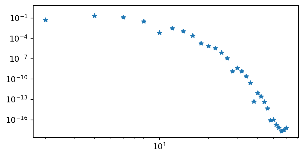
Implementation using Shenfun
from shenfun import FunctionSpace, TestFunction, TrialFunction, inner, Dx= 60 = FunctionSpace(N+ 3 , 'L' , bc= (0 , 0 )) # Chooses {P_j-P_{j+2}} basis = TrialFunction(VN)= TestFunction(VN)= inner(Dx(u, 0 , 1 ), Dx(v, 0 , 1 ))= inner(- f, v)= S.solve(b.copy())= plt.figure(figsize= (6 , 3 ))0 , N+ 1 , 2 ), abs (uh[:- 2 :2 ]), '*' );
Inhomogeneous Poisson
\[
\begin{align}
u''(x) &= f(x), \quad x \in (-1, 1) \\
u(-1) &= a, u(1) = b
\end{align}
\]
How to handle the inhomogeneous boundary conditions?
Use homogeneous \(\tilde{u}_N \in V_N\) and a boundary function \(B(x)\)
\[
u_N(x) = B(x) + \tilde{u}_N(x)
\]
where \(B(-1) = a\) and \(B(1) = b\) such that
\[
u_N(-1)=B(-1)=a \quad \text{and} \quad u_N(1) = B(1) = b
\]
A function that satisfies this in the current domain is
\[
B(x) = \frac{b}{2}(1+x) + \frac{a}{2}(1-x)
\]
Solve Poisson
Insert for \(u_N\) into \((R_N, v) = 0\) :
\[
\Big( (B(x)+\tilde{u}_N)'' - f, v \Big) = 0
\]
Since \(B(x)\) is linear \(B''=0\) and we get the homogeneous problem
\[
\Big( \tilde{u}^{''}_N - f, v \Big) = 0
\]
Solve exactly as before for \(\tilde{u}_N\) and the solution will be in the end
\[
u_N(x) = B(x) + \tilde{u}_N
\]
Implementation
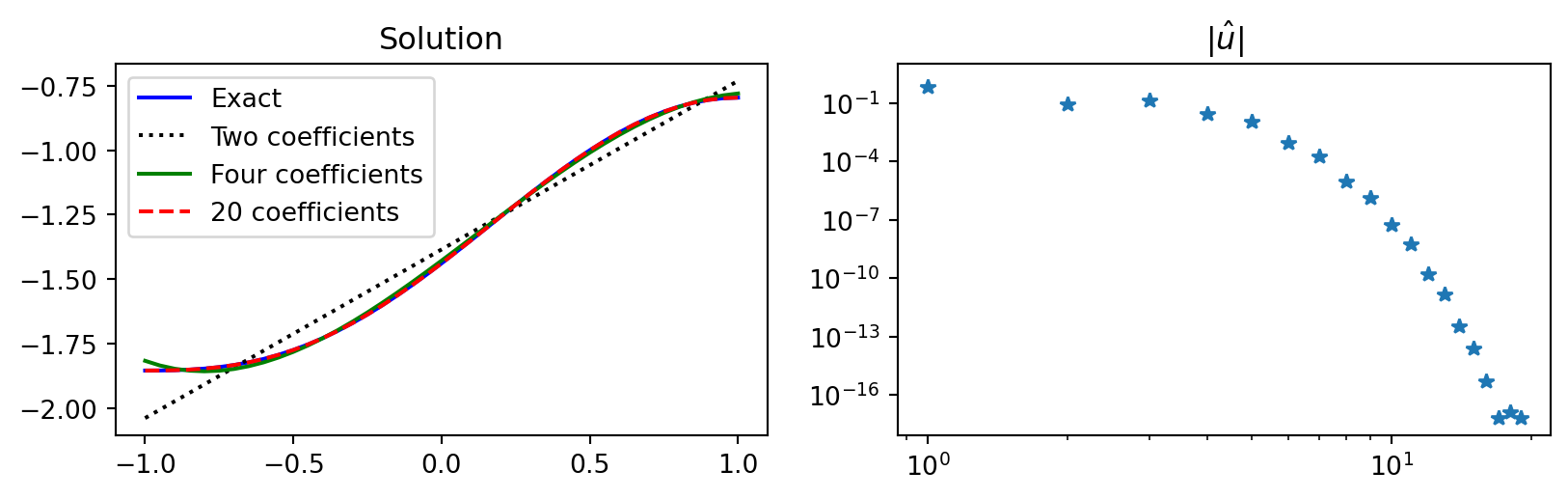
= sp.exp(sp.cos(x- 0.5 ))= ue.diff(x, 2 )= sp.lambdify(x, f)def uv(xj, j): return psi(j)(xj) * fl(xj)= lambda j: (- 1 / (4 * j+ 6 ))* quad(uv, - 1 , 1 , args= (j,))[0 ]= 30 = [uhat(k) for k in range (N)]= ue.subs(x, - 1 ), ue.subs(x, 1 )= b* (1 + x)/ 2 + a* (1 - x)/ 2 = 50 = np.linspace(- 1 , 1 , M+ 1 )= np.polynomial.legendre.legvander(xj, N+ 1 )= V[:, :- 2 ] - V[:, 2 :]= sp.lambdify(x, B)(xj)= plt.subplots(2 , 1 , figsize= (9 , 6 ))'b' ,1 ] @ np.array(utilde)[:1 ] + Bs, 'k:' ,@ np.array(utilde) + Bs, 'r--' )abs (np.array(utilde)), '*' )'Exact' , 'One coefficient' , f' { N} coefficients' ])'Solution' )r' $ | \ hat{u} | $ ' );
Neumann boundary conditions
\[
\begin{align}
u''(x) &= f(x), \quad x \in (-1, 1) \\
u'(\pm 1) &= 0
\end{align}
\]
This problem is ill-defined because if \(u\) is a solution, then \(u + c\) , where \(c\) is a constant, is also a solution!
If \(u(x)\) satisfies the above problem, then
\[
(u+c)'' = u'' + \cancel{c''} = f\quad \text{and} \quad (u+c)'(\pm 1) = u'(\pm 1) = 0
\]
We need an additional constraint! One possibility is then to require
\[
(u, 1) = \int_{\Omega} u(x) dx = c
\]
A well-defined Neumann problem
\[
\begin{align}
u''(x) &= f(x), \quad x \in (-1, 1) \\
u'(\pm 1) &= 0 \\
(u, 1) &= c
\end{align}
\]
How about basis functions?
If we choose basis functions \(\psi_j\) that satisfy
\[
\psi'_j(\pm 1) = 0, \quad j=0, 1, \ldots
\]
then
\[
u'_N(\pm 1) = \sum_{j=0}^N \hat{u}_j \psi'_j(\pm 1) = 0
\]
Neumann basis functions
Simplest possibility
\[
\psi_j = \cos(\pi j (x+1) / 2)
\]
Easy to see that \(\psi'_j(x) = -j/2\sin(j(x+1)/2)\) and thus \(\psi'_j(\pm 1) = 0\) . However, we also get that all odd derivatives are zero
\[
\frac{d^{2n+1} \psi_j}{dx^{2n+1}}(\pm 1) = 0, \quad n=0, 1, \ldots
\]
Lets try to find a basis function using Legendre polynomials instead
\[
\psi_j = P_j + b(j) P_{j+1} + a(j) P_{j+2}
\]
and try to find \(a(j)\) and \(b(j)\) such that \(\psi'_j(\pm 1) = 0\) .
Composite Legendre Neumann basis
\[
\psi_j = P_j + b(j)P_{j+1} + a(j) P_{j+2}
\]
\(\text{Using boundary conditions:} \quad P'_j(-1) = \frac{j(j+1)}{2}(-1)^j \quad \text{and} \quad P'_j(1) = \frac{j(j+1)}{2}\)
We have two conditions and two unknowns
\[\small
\begin{align}
\psi'_j(-1) &= P'_j(-1) + b(j)P'_{j+1}(-1) + a(j) P'_{j+2}(-1) \\
&= \left(\frac{j(j+1)}{2}-b(j)\frac{(j+1)(j+2)}{2} +a(j)\frac{(j+2)(j+3)}{2}\right)(-1)^j = 0
\end{align}
\]
\[ \small
\psi'_j(1) = \left(\frac{j(j+1)}{2} + b(j) \frac{(j+1)(j+2)}{2}+a(j)\frac{(j+2)(j+3)}{2}\right) = 0
\]
Solve the two equations to find \(a(j), b(j)\) and thus the Neumann basis function \(\psi_j\) :
\[
b(j)=0, \, a(j) = - \frac{j(j+1)}{(j+2)(j+3)} \longrightarrow \boxed{\psi_j = P_j - \frac{j(j+1)}{(j+2)(j+3)} P_{j+2}}
\]
Solve Neumann problem
Use the functionspace
\[
V_N = \text{span}\Big \{P_j - \frac{j(j+1)}{(j+2)(j+3)} P_{j+2} \Big \}_{j=0}^N
\]
and try to find \(u_N \in V_N\) .
However, we remember also the constraint and that
\[
(u, 1) = c \rightarrow (u_N, P_0)= c
\]
since \(\psi_0 = P_0 = 1\) . Insert for \(u_N\) and use orthogonality of Legendre polynomials to get
\[
\Big(\sum_{j=0}^N \hat{u}_j (P_j - \frac{j(j+1)}{(j+2)(j+3)} P_{j+2}), P_0\Big) = (P_0, P_0) \hat{u}_0 = 2 \hat{u}_0 = c
\]
So we already know that \(\hat{u}_0=c/2\) and only have unknowns \(\{\hat{u}_{j}\}_{j=1}^N\) left!
Solve Neumann with Galerkin
Define
\[
\tilde{V}_N = \text{span}\Big\{P_j - \frac{j(j+1)}{(j+2)(j+3)} P_{j+2}\Big\}_{j=1}^N (= V_N \backslash \{P_0\})
\]
With Galerkin: Find \(\tilde{u}_N \in \tilde{V}_N (= \sum_{j=1}^N \hat{u}_j \psi_j)\) such that
\[
(\tilde{u}^{''}_N - f, v) = 0, \quad \forall \, v \in \tilde{V}_N
\]
and use in the end
\[
u_N = \hat{u}_0 + \tilde{u}_N = \sum_{j=0}^N \hat{u}_j \psi_j
\]
The linear algebra problem
We need to solve
\[
\sum_{j=1}^N(\psi^{''}_j, \psi_i) \hat{u}_j = (f, \psi_i), \quad i=1,2, \ldots, N
\]
The stiffness matrix for Neumann
\[
(\psi^{''}_j, \psi_i) = -(\psi^{'}_j, \psi^{'}_i) = (\psi_j, \psi^{''}_i)
\]
is fortunately diagonal (derivation later) and we can easily solve for \(\{\hat{u}_i\}_{i=1}^N\)
\[
(\psi^{''}_j, \psi_i) = a(j) (4j+6) \delta_{ij}
\]
\[
\longrightarrow \hat{u}_i = \frac{(f, \psi_i)}{a(i)(4i+6)}, \quad i = 1, 2, \ldots, N
\]
Derivation of \((\psi^{''}_j, \psi_i)\)
There is a series expansion for the second derivative \(P^{''}_j\)
\[
P^{''}_j = \sum_{\substack{k=0 \\ k+j \text{ even}}}^{j-2}c(k, j) P_k, \, \text{where}\, c(k, j) = (k+1/2)(j(j+1)-k(k+1)) \tag{1}
\]
Hence \(P^{''}_N+a(N)P^{''}_{N+2}\) is a Legendre series ending at \(a(N)c(N-2, N)P_N\) . Consider
\[
\Big(P^{''}_j+a(j)P^{''}_{j+2}, \, P_i + a(i)P_{i+2} \Big)
\]
Based on the orthogonality \((P_i, P_j)=\frac{2}{2j+1}\delta_{ij}\) and (1) we get that
If \(i>j\) then \(\small(P^{''}_j+a(j)P^{''}_{j+2}, P_i + a(i)P_{i+2})=0\) since \(\small P^{''}_{j+2}=\sum_{k=0}^j c(k,j) P_k\)
If \(i< j\) then \(\small (P^{''}_j+a(j)P^{''}_{j+2}, P_i + a(i)P_{j+2})=0\) due to symmetry \((\psi^{''}_j, \psi_i) = (\psi_j, \psi^{''}_i)\)
Hence \(\Big(P^{''}_j+a(j)P^{''}_{j+2}, \, P_i + a(i)P_{i+2} \Big)\) is diagonal!
Compute \((\psi^{''}_i, \psi_i)\)
Using again the expression \(P^{''}_i = \sum_{k=0}^{i-2} c(k, i) P_{k}\)
\[ \small
\begin{multline}
\Big(P^{''}_i+a(i)P^{''}_{i+2}, P_i+a(i)P_{i+2}\Big) = \\ \cancel{(P^{''}_i, P_i)} + \cancel{a(i)(P^{''}_i, P_{i+2})} + a(i)(P^{''}_{i+2}, P_i) + \cancel{a^2(i)(P^{''}_{i+2}, P_{i+2})}
\end{multline}
\]
All cancellations because of orthogonality and \(P^{''}_i = \sum_{k=0}^{i-2} (\cdots) P_{k}\)
\[ \small
\begin{align}
a(i)(P^{''}_{i+2}, P_i) &= a(i) \sum_{\substack{k=0 \\ k+i \text{ even}}}^{i} \Big( (k+1/2)((i+2)(i+3)-k(k+1))P_k, \, P_i \Big) \\
&= a(i)(i+1/2)((i+2)(i+3)-i(i+1)) (P_i, P_i) \\
&= a(i)(4i+6)
\end{align}
\]
Hence we get the stiffness matrix
\[
(\psi^{''}_j, \psi_i) = a(i) (4i+6) \delta_{ij}
\]
Implementation
Use manufactured solution that we know satisfies the boundary conditions
\[
u(x) = \int (1-x^2)\cos (x-1/2)dx
\]
= sp.integrate((1 - x** 2 )* sp.cos(x- sp.S.Half), x)= ue.diff(x, 2 ) # manufactured f = sp.integrate(ue, (x, - 1 , 1 )).n() # constraint c = lambda j: Leg.basis(j)- j* (j+ 1 )/ ((j+ 2 )* (j+ 3 ))* Leg.basis(j+ 2 )= sp.lambdify(x, f)def uv(xj, j): return psi(j)(xj) * fj(xj)def a(j): return - j* (j+ 1 )/ ((j+ 2 )* (j+ 3 ))= lambda j: 1 / (a(j)* (4 * j+ 6 ))* quad(uv, - 1 , 1 , args= (j,))[0 ]= 30 ; uh = np.zeros(N); uh[0 ] = c/ 2 1 :] = [uhat(k) for k in range (1 , N)]
More about Neumann boundary conditions
We have used basis functions that satisfied
\[
\psi^{'}_j(\pm 1) = 0
\]
However, this was not strictly necessary! Neumann boundary conditions are often called natural conditions and we can implement them directly in the variational form:
\[
(\psi^{''}_j, \psi_i) = -(\psi^{'}_j, \psi{'}_i) + [\psi^{'}_j \psi_i]_{-1}^{1}
\]
Enforce boundary conditions weakly using \(\psi^{'}_j(-1)=a, \psi^{'}_j(1)=b\) :
\[
(\psi^{''}_j, \psi_i) = -(\psi^{'}_j, \psi{'}_i) + b \psi_i(1) - a \psi_i(-1)
\]
Homogeneous Neumann (\(a=b=0\) ):
\[
(\psi^{''}_j, \psi_i) = -(\psi^{'}_j, \psi{'}_i)
\]
Implementation
Using basis function \(\psi_j(x) = P_j(x)\) that have \(\psi^{'}_j(\pm 1) \ne 0\)
= lambda j: Leg.basis(j)def uf(xj, j): return psi(j)(xj) * fj(xj)def uv(xj, i, j): return - psi(i).deriv(1 )(xj) * psi(j).deriv(1 )(xj)= lambda j: quad(uf, - 1 , 1 , args= (j,))[0 ]= 20 # Compute the stiffness matrix (not diagonal) = np.zeros((N, N))for i in range (1 , N):for j in range (i, N):= quad(uv, - 1 , 1 , args= (i, j))[0 ]= S[i, j]0 , 0 ] = 1 # To fix constraint uh[0] = c/2 = np.zeros(N); fh[0 ] = c/ 2 1 :] = [fhat(k) for k in range (1 , N)]= np.array(fh, dtype= float )= np.linalg.solve(S, fh)
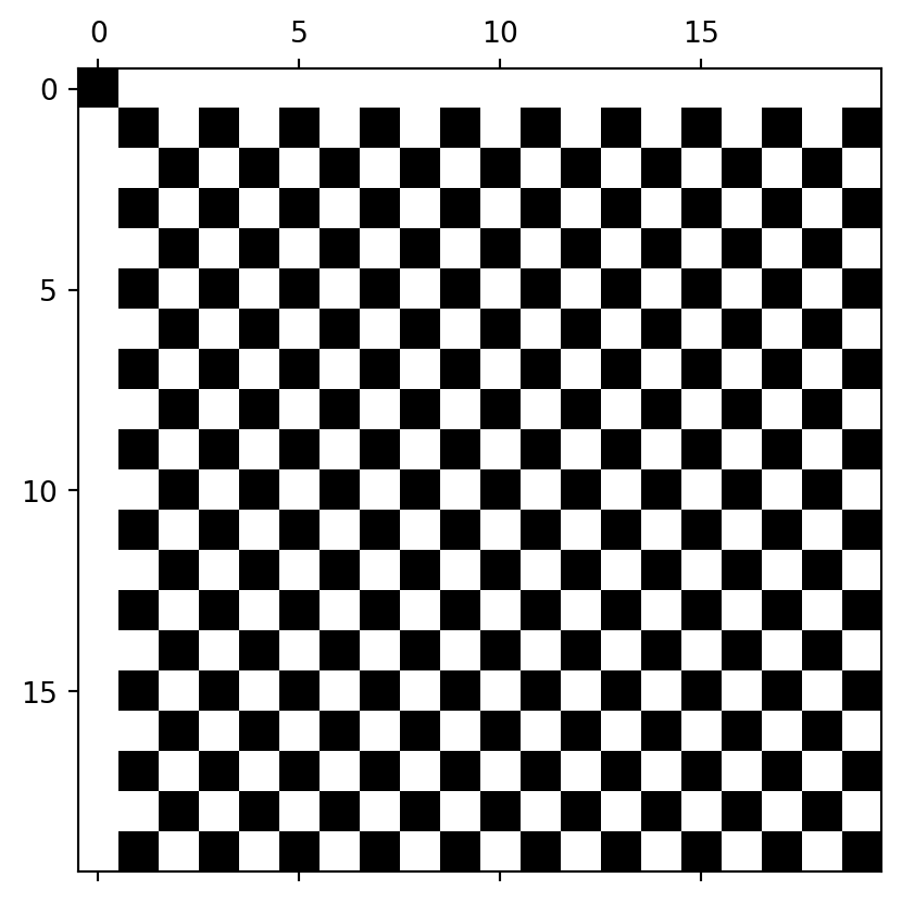
Dense stiffness matrix \((\psi'_j, \psi'_i)\)
Using basis function \(\psi_j = P_j\) leads to a dense stiffness matrix
and thus the need for the linear algebra solve \(\boldsymbol{\hat{u}} = S^{-1} \boldsymbol{f}\)
= np.linalg.solve(S, fh)
Chebyshev basis functions
Exactly the same approach as for Legendre, only with a weighted inner product \[
(u, v)_{\omega} = \int_{-1}^1 \frac{u v}{\sqrt{1-x^2}}dx
\]
For Dirichlet boundary conditions: Find \(u_N \in V_N = \text{span}\{T_i-T_{i+2}\}_{i=0}^N\) such that \[
(\mathcal{R}_N, v)_{\omega} = 0, \quad \forall \, v \in V_N
\] The basis functions \(\psi_i=T_i-T_{i+2}\) satisfy \(\psi_i(\pm 1)=0\) .
For Neumann boundary conditions, the basis functions are slightly different since \[
T'_k(-1) = (-1)^{k+1} k^2 \quad \text{and} \quad T'_{k}(1) = k^2
\] The basis functions \(\phi_k = T_{k} - \left(\frac{k}{k+2}\right)^2 T_{k+2}\) satisfy \(\phi'_k(\pm 1) = 0\) .
Inhomogeneous boundary conditions are handled like for Legendre with the same boundary function \(B(x)\) .
Collocation
Consider the Dirichlet problem
\[
\begin{align}
u''(x) &= f(x), \quad x \in (-1, 1) \\
u(-1) = a \quad &\text{and} \quad u(1) = b
\end{align}
\]
To solve this problem with collocation we use a mesh \(\boldsymbol{x}=\{x_i\}_{i=0}^N\) , where \(x_0=-1\) and \(x_N=1\) . The solution, using Lagrange polynomials, is
\[
u_N(x) = \sum_{i=0}^N \hat{u}_i \ell_i(x)
\]
We then require that the following \(N+1\) equations are satisfied
\[
\begin{align}
\mathcal{R}_N(x_i) &= 0, \quad i=1, 2, \ldots, N-1 \\
u(x_0) = a \quad &\text{and} \quad u(x_N) = b
\end{align}
\]
where \(\mathcal{R}_N(x) = u^{''}_N(x)-f(x)\) .
Solve by inserting for \(u_N\) in \(\mathcal{R}_N\)
We get the \(N-1\) equations for \(\{\hat{u}_j\}_{j=1}^{N-1}\)
\[
\sum_{j=0}^N \hat{u}_j \ell''_j(x_i) = f(x_i), \quad i = 1, 2, \ldots, N-1
\]
in addition to the boundary conditions: \(\hat{u}_0=u_N(x_0)=a\) and \(\hat{u}_N=u_N(x_N)=b\) .
The matrix \(D^{(2)} = (d^{(2)}_{ij})=(\ell^{''}_j(x_i))_{i,j=0}^N\) is dense. How do we compute it?
Using the Sympy Lagrange functions is numerically unstable
The main advantage of the Barycentric approach is numerical stability
And we can obtain the derivative matrix \(d_{ij} = \ell'_j(x_i)\) as
\[
\begin{align*}
d_{ij} &= \frac{w_j}{w_i(x_i-x_j)}, \quad i \, \neq j, \\
d_{ii} &= -\sum_{\substack{j=0 \\ j \ne i}}^N d_{ij}.
\end{align*}
\]
from scipy.interpolate import BarycentricInterpolatordef Derivative(xj):= BarycentricInterpolator(xj).wi= w[None , :] / w[:, None ]= xj[:, None ]- xj[None , :]1 )= W / X0 )- np.sum (D, axis= 1 ))return D
W is the matrix with items \(w_j / w_i\) . \(w_i\) varies along the first axis and is thus w[:, None]. \(w_j\) varies along the second axis and is w[None, :]. Likewise \(x_i\) is xj[:, None] and \(x_j\) is xj[None, :]
Higher order derivative matrices \(d^{n}_{ij} = \ell^{(n)}_j(x_i)\) can be computed recursively
\[
\begin{align*}
d^{(n)}_{ij} &= \frac{n}{x_i-x_j}\left(\frac{w_j}{w_i} d^{(n-1)}_{ii} - d^{(n-1)}_{ij} \right) \\
d^{(n)}_{ii} &= -\sum_{\substack{j=0 \\ j \ne i}}^N d^{(n)}_{ij}
\end{align*}
\]
def PolyDerivative(xj, m):= BarycentricInterpolator(xj).wi * (2 * (len (xj)- 1 ))= w[None , :] / w[:, None ]= xj[:, None ]- xj[None , :]1 )= W / X0 )- np.sum (D, axis= 1 ))if m == 1 : return D= np.zeros_like(D)for k in range (2 , m+ 1 ):= k / X * (W * D.diagonal()[:, None ] - D)0 )- np.sum (D2, axis= 1 ))= D2return D2
Use Chebyshev points for spectral accuracy
\[
x_i = \cos(i \pi / N)
\]
The barycentric weights are then simply
\[
w_i = (-1)^{i} c_i, \quad c_i = \begin{cases} 0.5 \quad i=0 \text{ or } i = N \\
1 \quad \text{ otherwise}
\end{cases} \tag{1}
\]
= 8 = np.cos(np.arange(N+ 1 )* np.pi/ N)= BarycentricInterpolator(xj).wi * 2 * N
array([ 0.5, -1. , 1. , -1. , 1. , -1. , 1. , -1. , 0.5])
The weights are only relative, so we have here scaled by \(2N\) to get (1)
And then we solve any equation by replacing the ordinary derivatives with derivative matrices
\[
\begin{align}
u''(x) &= f(x), \quad x \in (-1, 1) \\
u(-1) = a \quad &\text{and} \quad u(1) = b
\end{align}
\]
Let \(d^{(2)}_{ij} = \ell^{''}_j(x_i)\) for all \(i=1, \ldots, N-1\) , ident the first and last rows of \(D^{(2)}\) and set \(f_0=a\) and \(f_N=b\) . Solve
\[
\sum_{j=0}^N d^{(2)}_{ij} \hat{u}_j = f_i, \quad i=0, 1, \ldots, N
\]
Matrix form using \(\boldsymbol{\hat{u}} = (\hat{u}_j)_{j=0}^N\) and \(\boldsymbol{f} = (f_j)_{j=0}^N\)
\[
D^{(2)} \boldsymbol{\hat{u}} = \boldsymbol{f}
\]
\[
\boldsymbol{\hat{u}} = (D^{(2)})^{-1} \boldsymbol{f}
\]
Implementation for Poisson’s equation
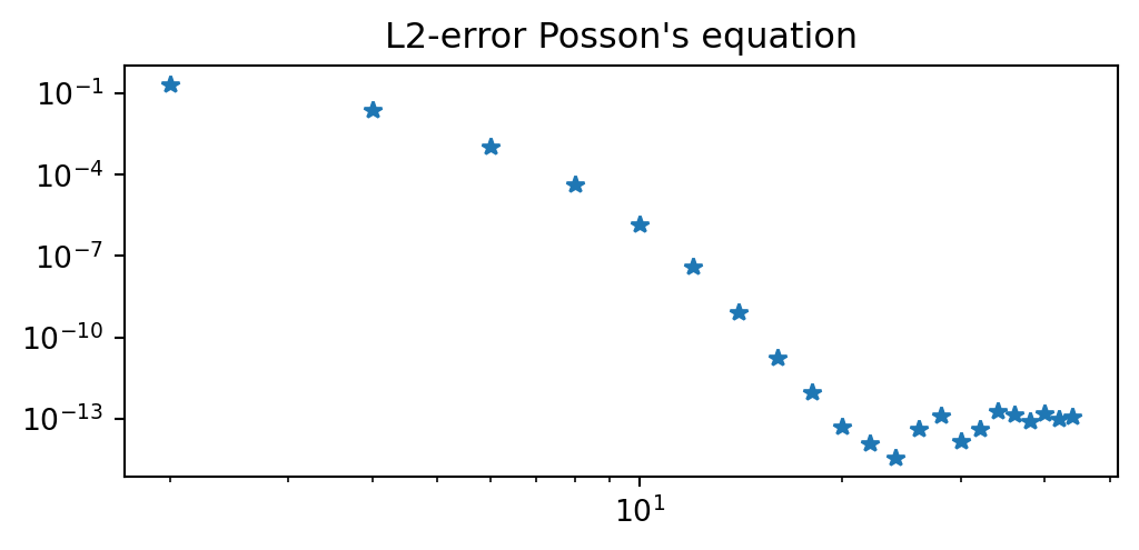
def poisson_coll(N, f, bc= (0 , 0 )):= np.cos(np.arange(N+ 1 )* np.pi/ N)[::- 1 ]= PolyDerivative(xj, 2 ) # Get second derivative matrix 0 , 0 ] = 1 ; D2[0 , 1 :] = 0 # ident first row - 1 , - 1 ] = 1 ; D2[- 1 , :- 1 ] = 0 # ident last row = np.zeros(N+ 1 )1 :- 1 ] = sp.lambdify(x, f)(xj[1 :- 1 ])0 ], fh[- 1 ] = bc # Fix boundary conditions = np.linalg.solve(D2, fh)return uh, D2def l2_error(uh, ue):= sp.lambdify(x, ue)= len (uh)- 1 = np.cos(np.arange(N+ 1 )* np.pi/ N)[::- 1 ]= BarycentricInterpolator(np.cos(np.arange(N+ 1 )* np.pi/ N)[::- 1 ], yi= uh)= 4 * len (uh) # Use denser mesh to compute L2-error = np.linspace(- 1 , 1 , N+ 1 )return np.sqrt(np.trapz((uj(xj)- L(xj).astype(float ))** 2 , dx= 2. / N))
= sp.exp(sp.cos(x- 0.5 ))= ue.diff(x, 2 )= ue.subs(x, - 1 ), ue.subs(x, 1 )= []for N in range (2 , 46 , 2 ):= poisson_coll(N, f, bc= bc)= plt.figure(figsize= (6 , 2.5 ))2 , 46 , 2 ), err, '*' )"L2-error Posson's equation" );
Summary
Find \(u_N \in V_N\) such that \[(\mathcal{L}(u_N) - f, v) = (\mathcal{R}_N, v) = 0 \quad \forall v \in W\]
Differential equations are solved using the method of weighted residuals
Galerkin (\(W=V_N\) )
Least squares (\(W = \text{span}\{\frac{\partial \mathcal{R}_N}{\partial \hat{u}_i}\}_{i=0}^N\) )
Collocation (\(v = \delta(x-x_i)\) )
Same approach as function approximation, but assembling matrices is more work!
Basis functions chosen to satisfy homogeneous boundary conditions (either Dirichlet or Neumann) and then a lifting function \(B(x)\) handles nonzero conditions \(u_N(x) = \sum_{i=0}^N \hat{u}_i \psi_i(x) + B(x)\)
Multi-dimensional problems (PDEs) can be solved using tensor-product spaces, vectorization and the Kronecker product (see lecture notes).