The finite difference method
MATMEK-4270
Initial or Boundary Value Problems
The second-order differential equation
\[ u''(t) + au'(t) + bu(t) = f(t), \quad t \in [0, T] \]
is classified as either an IVP or a BVP based on boundary/initial conditions.
IVP
- Typically specifies \(u(0)\) and \(u'(0)\)
- Explicit recurrence relations, no use of linear algebra
- Can use the finite difference or similar methods for discretization
BVP
- Typically specifies \(u(0)\) and \(u(T)\) or \(u'(0)\) and \(u'(T)\)
- Implicit linear algebra methods
- Can use the finite difference or similar methods for discretization
Similar characteristics for higher-order differential equations. IVP specifies all conditions at initial time.
The explicit IVP approach simply computes \(u^{n+1}\) from \(u^n, u^{n-1}\)…
For example, the exponential decay problem with initial condition
\[ u' + au = 0, t \in (0, T], \, u(0)=I. \]
is discretized as
\[ u^{n+1} = \frac{1 - (1-\theta) a \Delta t}{1 + \theta a \Delta t} u^n = g u^n. \]
The solution vector \(\boldsymbol{u} = (u^0, u^1, \ldots, u^{N})\) is obtained from a recurrence algorithm
- \(u^0 = I\)
- for n = 0, 1, … , N-1
- Compute \(u^{n+1} = g u^n\)
Easy to understand and easy to solve. Equations are never assembled into matrix form. But may be unstable!
The BVP approach solves the difference equations by assembling matrices and vectors
Each row in the matrix-problem represents one difference equation.
\[ A \boldsymbol{u} = \boldsymbol{b} \]
For the exponential decay problem the matrix problem looks like
\[ \underbrace{ \begin{bmatrix} 1 & 0 & 0 & 0 & 0 \\ -g & 1 & 0 & 0 & 0 \\ 0 & -g & 1 & 0 & 0 \\ 0 & 0 & -g & 1 & 0 \\ 0 & 0 & 0 & -g & 1 \end{bmatrix}}_{A} \underbrace{\begin{bmatrix} u^0 \\ u^1 \\ u^2 \\ u^3 \\ u^4 \end{bmatrix}}_{\boldsymbol{u}} = \underbrace{\begin{bmatrix} I \\ 0 \\ 0 \\ 0 \\ 0 \end{bmatrix}}_{\boldsymbol{b}} \]
Understand that the matrix problem is the same as the recurrence
\[ \underbrace{ \begin{bmatrix} 1 & 0 & 0 & 0 & 0 \\ -g & 1 & 0 & 0 & 0 \\ 0 & -g & 1 & 0 & 0 \\ 0 & 0 & -g & 1 & 0 \\ 0 & 0 & 0 & -g & 1 \end{bmatrix}}_{A} \underbrace{\begin{bmatrix} u^0 \\ u^1 \\ u^2 \\ u^3 \\ u^4 \end{bmatrix}}_{\boldsymbol{u}} = \underbrace{\begin{bmatrix} I \\ 0 \\ 0 \\ 0 \\ 0 \end{bmatrix}}_{\boldsymbol{b}} \]
simply means
\[ \begin{align} u^0 &= I \\ -g u^0 + u^1 &= 0 \\ -g u^1 + u^2 &= 0 \\ \vdots \end{align} \]
Still explicit since matrix is lower triangular. But problem is assembled into matrix form.
Solve matrix problem
The matrix problem
\[ A \boldsymbol{u} = \boldsymbol{b} \]
is solved as
\[ \boldsymbol{u} = A^{-1} \boldsymbol{b} \]
There are many different ways to achieve this. We will not be very concerned with how in this course.
Assemble matrix problem
Assemble
Solve and compare with recurrence
Recurrence:
Matrix
Ok, no difference. There’s really no advantage of assembling the explicit exponential decay problem.
But which is faster?
Try to speed up by computing the inverse
A unit lower triangular matrix has a unit lower triangular inverse
[[1. 0. 0. 0. 0. 0. 0. 0. 0. ]
[0.333 1. 0. 0. 0. 0. 0. 0. 0. ]
[0.111 0.333 1. 0. 0. 0. 0. 0. 0. ]
[0.037 0.111 0.333 1. 0. 0. 0. 0. 0. ]
[0.012 0.037 0.111 0.333 1. 0. 0. 0. 0. ]
[0.004 0.012 0.037 0.111 0.333 1. 0. 0. 0. ]
[0.001 0.004 0.012 0.037 0.111 0.333 1. 0. 0. ]
[0. 0.001 0.004 0.012 0.037 0.111 0.333 1. 0. ]
[0. 0. 0.001 0.004 0.012 0.037 0.111 0.333 1. ]]Try to speed up by computing the inverse
A unit lower triangular matrix has a unit lower triangular inverse
Now solve directly using \(A^{-1}\)
Compare with previous - still the same
Until we try Numba on the explicit solver
import numba as nb
@nb.jit
def nbreccsolve(u, N, I, g):
u[0] = I
for n in range(N):
  u[n+1] = g * u[n]
nbreccsolve(u, N, I, g)
%timeit -n 100 nbreccsolve(u, N, I, g)124 ns ± 9.72 ns per loop (mean ± std. dev. of 7 runs, 100 loops each)Bottom line - explicit marching methods are very fast! Unfortunately, they may be unstable and cannot be used for BVPs.
The BV vibration problem
\[ u'' + \omega^2 u = 0,\, t \in (0, T) \quad u(0) = I, u(T) = I, \]
cannot be solved with recurrence, since it is not an initial value problem.
However, we can solve this problem using a central finite difference for all internal points \(n=1, 2, \ldots, N-1\)
\[ \frac{u^{n+1}-2u^n+u^{n-1}}{\Delta t^2} + \omega^2 u^n = 0. \]
This leads to an implicit linear algebra problem, because the equation for \(u^n\) (above) depends on \(u^{n+1}\)!
Vibration on matrix form
The matrix problem is now, using \(g = 2-\omega^2 \Delta t^2\),
\[ \begin{bmatrix} 1 & 0 & 0 & 0 & 0 & 0 & 0 \\ 1 & -g & 1 & 0 & 0 & 0 & 0 \\ 0 & 1 & -g & 1 & 0 & 0 & 0 \\ 0 & 0 & 1 & -g & 1 & 0 & 0 \\ 0 & 0 & 0 & 1 & -g & 1 & 0 \\ 0 & 0 & 0 & 0 & 1 & -g & 1 \\ 0 & 0 & 0 & 0 & 0 & 0 & 1 \end{bmatrix} \begin{bmatrix} u^0 \\ u^1 \\ u^2 \\ u^3 \\ u^4 \\ u^5 \\ u^6 \end{bmatrix} = \begin{bmatrix} I \\ 0 \\ 0 \\ 0 \\ 0 \\ 0 \\ I \end{bmatrix} \]
Note
- The matrix contains items both over and under the main diagonal, which characterizes an implicit method. Explicit marching method leads to lower triangular matrices.
- The first and last rows are modified in order to apply boundary conditions implicitly. More about that later.
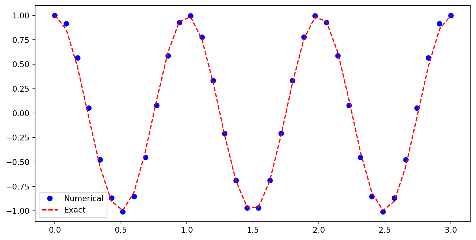
Assemble and solve the implicit BVP
T, N, I, w = 3., 35, 1., 2*np.pi
dt = T/N
g = 2 - w**2*dt**2
A = sparse.diags([1, -g, 1], np.array([-1, 0, 1]), (N+1, N+1), 'lil')
b = np.zeros(N+1)
A[0, :3] = 1, 0, 0    # Fix first row
A[-1, -3:] = 0, 0, 1  # Fix last row
b[0], b[-1] = I, I
u2 = sparse.linalg.spsolve(A.tocsr(), b)
t = np.linspace(0, T, N+1)
plt.figure(figsize=(10, 4))
plt.plot(t, u2, 'bo', t, I*np.cos(w*t), 'r--')
plt.legend(['Numerical', 'Exact']);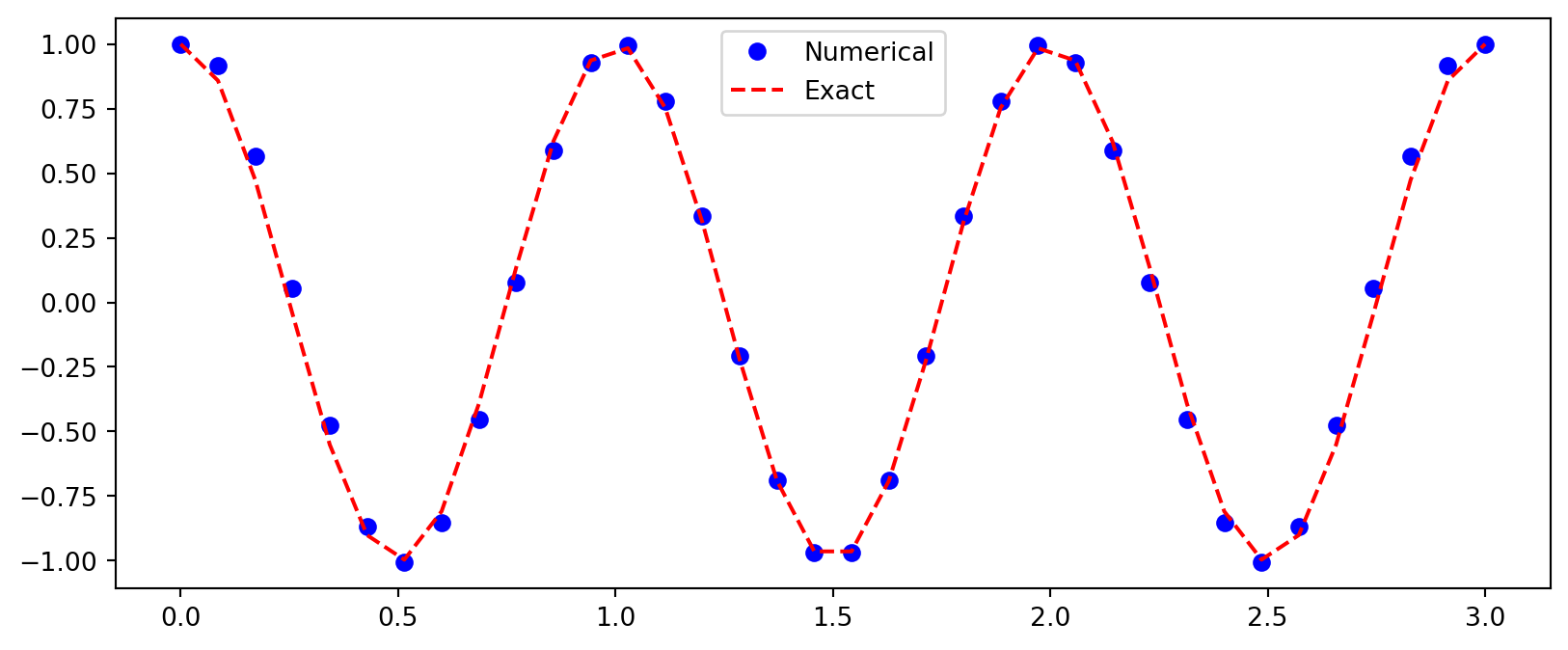
Implicit finite difference methods
Taylor expansions can be used to design finite difference methods of any order
For example, we can create two backward and two forward Taylor expansions starting from \(u^n=u(t_n)\)
\[ \small \begin{align*} (-2)\quad u^{n-2} &= u^n - 2h u' + \frac{2 h^2}{1}u'' - \frac{4 h^3}{3}u''' + \frac{2 h^4}{3}u'''' - \cdots \\ (-1)\quad u^{n-1} &= u^n - h u' + \frac{h^2}{2}u'' - \frac{h^3}{6}u''' + \frac{h^4}{24}u'''' - \cdots \\ (1)\quad u^{n+1} &= u^n + h u' + \frac{h^2}{2}u'' + \frac{h^3}{6}u''' + \frac{h^4}{24}u'''' + \cdots \\ (2)\quad u^{n+2} &= u^n + 2h u' + \frac{2 h^2}{1}u'' + \frac{4 h^3}{3}u''' + \frac{2 h^4}{3}u'''' + \cdots \end{align*} \]
Remember: \(u^{n+a} = u(t_{n+a})\) and \(t_{n+a} = (n+a)h\) and we use \(h=\Delta t\) for simplicity.
Add equations (-1) and (1) and isolate \(u''(t_n)\)
\[ \begin{equation*} u''(t_n) = \frac{u^{n+1}-2u^n + u^{n-1}}{h^2} + \frac{h^2}{12}u'''' + \end{equation*} \]
The FD stencil can be applied to the entire mesh
That is, we can compute \(\boldsymbol{u}^{(2)}=(u''(t_n))_{n=0}^{N}\) from the mesh function \(\boldsymbol{u} = (u(t_n))_{n=0}^N \in \mathbb{R}^{N+1}\) as
\[ \boldsymbol{u}^{(2)} = D^{(2)} \boldsymbol{u}, \]
where \(D^{(2)} \in \mathbb{R}^{N+1 \times N+1}\) is the second derivative matrix.
\[ \small \underbrace{ \begin{bmatrix} u^{(2)}_0 \\ u^{(2)}_1 \\ u^{(2)}_2 \\ \vdots \\ u^{(2)}_{N-2} \\ u^{(2)}_{N-1} \\ u^{(2)}_{N} \\ \end{bmatrix}}_{\boldsymbol{u}^{(2)}} = \underbrace{ \frac{1}{h^2} \begin{bmatrix} ? & ? & ? & ? & ? & ? & ? & ? \\ 1 & -2 & 1 & 0 & 0 & 0 & 0 & \cdots \\ 0 & 1 & -2 & 1 & 0 & 0 & 0 & \cdots \\ \vdots & & & \ddots & & & &\cdots \\ \vdots & 0 & 0 & 0 & 1& -2& 1& 0 \\ \vdots & 0 & 0& 0& 0& 1& -2& 1 \\ ? & ? & ? & ? & ? & ? & ? & ? \\ \end{bmatrix} }_{D^{(2)}} \underbrace{\begin{bmatrix} u^0 \\ u^1 \\ u^2 \\ \vdots \\ u^{N-1} \\ u^{N-1} \\ u^{N} \end{bmatrix}}_{\boldsymbol{u}} \]
How about the boundary nodes?
\[ \small \underbrace{ \begin{bmatrix} u^{(2)}_0 \\ u^{(2)}_1 \\ u^{(2)}_2 \\ \vdots \\ u^{(2)}_{N-2} \\ u^{(2)}_{N-1} \\ u^{(2)}_{N} \\ \end{bmatrix}}_{\boldsymbol{u}^{(2)}} = \underbrace{ \frac{1}{h^2} \begin{bmatrix} ? & ? & ? & ? & ? & ? & ? & ? \\ 1 & -2 & 1 & 0 & 0 & 0 & 0 & \cdots \\ 0 & 1 & -2 & 1 & 0 & 0 & 0 & \cdots \\ \vdots & & & \ddots & & & &\cdots \\ \vdots & 0 & 0 & 0 & 1& -2& 1& 0 \\ \vdots & 0 & 0& 0& 0& 1& -2& 1 \\ ? & ? & ? & ? & ? & ? & ? & ? \\ \end{bmatrix} }_{D^{(2)}} \underbrace{\begin{bmatrix} u^0 \\ u^1 \\ u^2 \\ \vdots \\ u^{N-1} \\ u^{N-1} \\ u^{N} \end{bmatrix}}_{\boldsymbol{u}} \]
What to do with the first and last rows? The central stencils do not work here.
We still want to compute \(u_0^{(2)}=u''(t_0)\) and \(u_N^{(2)}=u''(t_N)\). How?
Forward and backward stencils will do
We can do a forward difference at \(n=0\)
Remember: \[ \small \begin{align*} (1)\quad u^{n+1} &= u^n + h u' + \frac{h^2}{2}u'' + \frac{h^3}{6}u''' + \frac{h^4}{24}u'''' + \cdots \\ (2)\quad u^{n+2} &= u^n + 2h u' + \frac{2 h^2}{1}u'' + \frac{4 h^3}{3}u''' + \frac{2 h^4}{3}u'''' + \cdots \end{align*} \]
Subtract 2 times Eq. (1) from Eq. (2) and rearrange
\[\small (2)-2(1): \, u^{n+2} - 2u^{n+1} = -u^n + \frac{h^2}{1}u'' + h^3 u''' + \frac{7 h^4}{12}u'''' + \]
Rearrange to isolate a first order accurate stencil for \(u''(0)\)
\[\small u''(0) = \frac{u^{2}-2u^{1}+u^0}{h^2} - \color{red} h \color{black} u'''(0) - \frac{7 h^2}{12}u''''(0) + \]
We can do a backward difference at \(n=N\)
Use two backward Taylor expansions:
\[ \small \begin{align*} (-2)\quad u^{n-2} &= u^n - 2 h u' + \frac{2 h^2}{1}u'' - \frac{4 h^3}{3}u''' + \frac{2 h^4}{3}u'''' - \cdots \\ (-1)\quad u^{n-1} &= u^n - h u' + \frac{h^2}{2}u'' - \frac{h^3}{6}u''' + \frac{h^4}{24}u'''' - \cdots \\ \end{align*} \]
Subtract 2 times Eq. (-1) from Eq. (-2) and rearrange
\[\small (-2)-2(-1): \, u^{n-2} - 2u^{n-1} = -u^n + \frac{h^2}{1}u'' - h^3 u''' + \frac{7 h^4}{12}u'''' + \]
Rearrange to isolate a first order accurate backward stencil for \(u''(T)\)
\[\small u''(T) = \frac{u^{N-2}-2u^{N-1}+u^N}{h^2} - \color{red} h \color{black} u'''(T) - \frac{7 h^2}{12}u''''(T) + \]
We get a second derivative matrix
\[ D^{(2)} = \frac{1}{h^2} \begin{bmatrix} 1 & -2 & 1 & 0 & 0 & 0 & 0 & 0 \\ 1 & -2 & 1 & 0 & 0 & 0 & 0 & \cdots \\ 0 & 1 & -2 & 1 & 0 & 0 & 0 & \cdots \\ \vdots & & & \ddots & & & &\cdots \\ \vdots & 0 & 0 & 0 & 1& -2& 1& 0 \\ \vdots & 0 & 0& 0& 0& 1& -2& 1 \\ 0 & 0 & 0 & 0 & 0 & 1 & -2 & 1 \\ \end{bmatrix} \]
but with merely first order accuracy at the boundaries. Can we do better?
Yes! Of course, just use more points near the boundaries!
Use three forward points \(\small u^{n+1}, u^{n+2}, u^{n+3}\) to get a second order forward stencil
\[ \small \begin{align*} (1)\quad u^{n+1} &= u^n + h u' + \frac{h^2}{2}u'' + \frac{h^3}{6}u''' + \frac{h^4}{24}u'''' + \cdots \\ (2)\quad u^{n+2} &= u^n + 2h u' + \frac{2 h^2}{1}u'' + \frac{4 h^3}{3}u''' + \frac{2 h^4}{3}u'''' + \cdots \\ (3)\quad u^{n+3} &= u^n + 3h u' + \frac{9 h^2}{2}u'' + \frac{9 h^3}{2}u''' + \frac{27 h^4}{8}u'''' + \cdots \\ \end{align*} \]
Now to eliminate both \(u'\) and \(u'''\) terms add the three equations as \(-(3) + 4\cdot(2) - 5\cdot(1)\) (don’t worry about how I know this yet)
\[ -(3)+4\cdot(2)-5\cdot(1): \, -u^{n+3}+4u^{n+2}-5u^{n+1} = -2 u^n + h^2 u'' - \frac{11 h^4}{12}u'''' + \]
Isolate \(u''(0)\)
\[ u''(0) = \frac{-u^{3} + 4u^{2} - 5u^{1} + 2u^0}{h^2} + \frac{11 \color{red} h^2 \color{black}}{12} u'''' + \]
Fully second order \(D^{(2)}\)
\[ D^{(2)} = \frac{1}{h^2} \begin{bmatrix} 2 & -5 & 4 & -1 & 0 & 0 & 0 & 0 \\ 1 & -2 & 1 & 0 & 0 & 0 & 0 & \cdots \\ 0 & 1 & -2 & 1 & 0 & 0 & 0 & \cdots \\ \vdots & & & \ddots & & & &\cdots \\ \vdots & 0 & 0 & 0 & 1& -2& 1& 0 \\ \vdots & 0 & 0& 0& 0& 1& -2& 1 \\ 0 & 0 & 0 & 0 & -1 & 4 & -5 & 2 \\ \end{bmatrix} \]
Assemble in Python
N = 8
dt = 0.5
T = N*dt
D2 = sparse.diags([1, -2, 1], np.array([-1, 0, 1]), (N+1, N+1), 'lil')
D2[0, :4] = 2, -5, 4, -1
D2[-1, -4:] = -1, 4, -5, 2
D2 *= (1/dt**2) # don't forget h
D2.toarray()*dt**2
array([[ 2., -5., 4., -1., 0., 0., 0., 0., 0.],
[ 1., -2., 1., 0., 0., 0., 0., 0., 0.],
[ 0., 1., -2., 1., 0., 0., 0., 0., 0.],
[ 0., 0., 1., -2., 1., 0., 0., 0., 0.],
[ 0., 0., 0., 1., -2., 1., 0., 0., 0.],
[ 0., 0., 0., 0., 1., -2., 1., 0., 0.],
[ 0., 0., 0., 0., 0., 1., -2., 1., 0.],
[ 0., 0., 0., 0., 0., 0., 1., -2., 1.],
[ 0., 0., 0., 0., 0., -1., 4., -5., 2.]])Apply matrix to a mesh function \(f(t_n) = t_n^2\)
Exact for all \(n\)!
Try with merely first order boundary
D21 = sparse.diags([1, -2, 1], np.array([-1, 0, 1]), (N+1, N+1), 'lil')
D21[0, :4] = 1, -2, 1, 0
D21[-1, -4:] = 0, 1, -2, 1
D21 *= (1/dt**2)
D21 @ f
array([2., 2., 2., 2., 2., 2., 2., 2., 2.])Still exact! Why?
Consider the forward first order stencil
\[ u''(0) = \frac{u^{2}-2u^{1}+u^0}{h^2} - \color{red} h u'''(0) \color{black} - \frac{7 h^2}{12}u''''(0) + \]
The leading error is \(h u'''(0)\) and \(u'''(0)\) is zero for \(u(t)=t^2\). The second order stencil captures the second order polynomial \(t^2\) exactly!
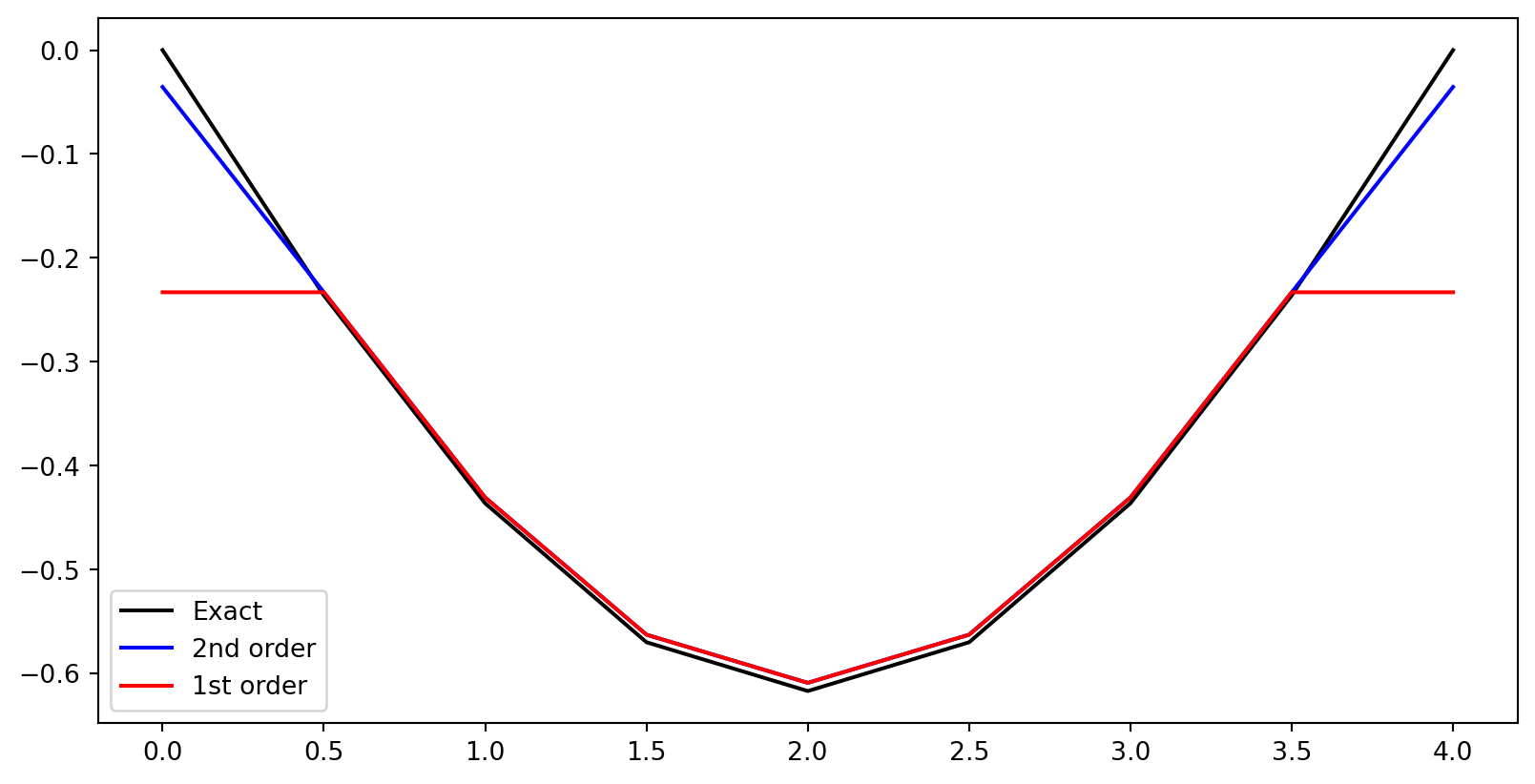
More challenging example
Let \(f(t) = \sin(\pi t / T)\) such that \(f''(t) = -(\pi/T)^2 f(t)\). Here none of the error terms will disappear and we see the effect of the poor first order boundary.
First derivative matrix
Lets create a similar matrix for a second order accurate single derivative.
\[ \small \begin{align} (-1)\quad u^{n-1} &= u^n - h u' + \frac{h^2}{2}u'' - \frac{h^3}{6}u''' + \frac{h^4}{24}u'''' + \cdots \\ (1)\quad u^{n+1} &= u^n + h u' + \frac{h^2}{2}u'' + \frac{h^3}{6}u''' + \frac{h^4}{24}u'''' + \cdots \end{align} \]
Here Eq. (1) minus Eq. (-1) leads to
\[ u'(t_n) = \frac{u^{n+1}-u^{n-1}}{2 h} + \frac{h^2}{6} u''' + \]
which is second order accurate.
The central scheme cannot be used for \(n=0\) or \(n=N\).
We use a forward scheme for \(n=0\)
\[ \small \begin{align} (1)\quad u^{n+1} &= u^n + h u' + \frac{h^2}{2}u'' + \frac{h^3}{6}u''' + \frac{h^4}{24}u'''' + \cdots \\ (2)\quad u^{n+2} &= u^n + 2h u' + \frac{2 h^2}{1}u'' + \frac{4 h^3}{3}u''' + \frac{2 h^4}{3}u'''' + \cdots \end{align} \]
From Eq. (1):
\[ u'(t_n) = \frac{u^{n+1}-u^n}{h} - \frac{\color{red}h\color{black}}{2}u'' - \]
Adding one more equation (2) we get second order: \(4\cdot (1) - (2)\) (Note that the terms with \(u''\) then cancel)
\[ u'(t_n) = \frac{-u^{n+2}+4u^{n+1}-3u^n}{2h} + \frac{\color{red}h^2\color{black}}{3}u''' + \]
With forward and backward on the edges we get a second order first derivative matrix
\[ \small D^{(1)} = \frac{1}{2 h}\begin{bmatrix} -3 & 4 & -1 & 0 & 0 & 0 & 0 & 0 \\ -1 & 0 & 1 & 0 & 0 & 0 & 0 & \cdots \\ 0 & -1 & 0 & 1 & 0 & 0 & 0 & \cdots \\ \vdots & & & \ddots & & & &\cdots \\ \vdots & 0 & 0 & 0 & -1& 0& 1& 0 \\ \vdots & 0 & 0& 0& 0& -1& 0& 1 \\ 0 & 0 & 0 & 0 & 0 & 1 & -4 & 3 \\ \end{bmatrix} \]
Is \(D^{(2)}\) the same as \(D^{(1)}D^{(1)}\)?
Is it the same to compute \(D^{(2)} \boldsymbol{u}\) as \(D^{(1)}(D^{(1)}\boldsymbol{u})\)?
Analytically, we know that \(u'' = \frac{d^2u}{dt^2} = \frac{d}{dt}\left(\frac{du}{dt}\right)\), but this is not necessarily so numerically.
array([[  5., -11.,   7.,  -1.,   0.,   0.,   0.,   0.,   0.],
       [  3.,  -5.,   1.,   1.,   0.,   0.,   0.,   0.,   0.],
       [  1.,   0.,  -2.,   0.,   1.,   0.,   0.,   0.,   0.],
       [  0.,   1.,   0.,  -2.,   0.,   1.,   0.,   0.,   0.],
       [  0.,   0.,   1.,   0.,  -2.,   0.,   1.,   0.,   0.],
       [  0.,   0.,   0.,   1.,   0.,  -2.,   0.,   1.,   0.],
       [  0.,   0.,   0.,   0.,   1.,   0.,  -2.,   0.,   1.],
       [  0.,   0.,   0.,   0.,   0.,   1.,   1.,  -5.,   3.],
       [  0.,   0.,   0.,   0.,   0.,  -1.,   7., -11.,   5.]])
This stencil is wider than \(D^{(2)}\), using neighboring points farther away. The central stencil is
\[ u''(t_n) = \frac{u^{n+2}-2u^{n}+u^{n-2}}{4h^2} \]
How accurate is \(D^{(1)}D^{(1)}\)?
Internal points
\[ \small \begin{align*} (-2)\quad u^{n-2} &= u^n - 2h u' + \frac{2 h^2}{1}u'' - \frac{4 h^3}{3}u''' + \frac{2 h^4}{3}u'''' - \cdots \\ (2)\quad u^{n+2} &= u^n + 2h u' + \frac{2 h^2}{1}u'' + \frac{4 h^3}{3}u''' + \frac{2 h^4}{3}u'''' + \cdots \end{align*} \]
Take Eq. (2) plus Eq. (-2)
\[ u^{n+2} + u^{n-2} = 2u^n + 4h^2 u'' + \frac{4h^4}{3}u'''' + \]
and
\[ u''(t_n) = \frac{u^{n+2}-2u^{n}+u^{n-2}}{4h^2} - \frac{h^2}{3}u'''' + \cdots \]
The stencil in the center (for \(1<n<N-1\)) of \(D^{(1)}D^{(1)}\) is second order!
How about boundaries?
We have obtained \(u''(t_1) = \frac{u^{n+2}+u^{n+1}-5u^{n}+3u^{n-1}}{4h^2}\). Compute the error in this stencil using one backward and two forward points
\[ \small \begin{align*} (-1)\quad u^{n-1} &= u^n - h u' + \frac{h^2}{2}u'' - \frac{h^3}{6}u''' + \frac{h^4}{24}u'''' - \cdots \\ (1)\quad u^{n+1} &= u^n + h u' + \frac{h^2}{2}u'' + \frac{h^3}{6}u''' + \frac{h^4}{24}u'''' + \cdots \\ (2)\quad u^{n+2} &= u^n + 2h u' + \frac{2 h^2}{1}u'' + \frac{4 h^3}{3}u''' + \frac{2 h^4}{3}u'''' + \cdots \end{align*} \]
Take Eq. \((2) + (1) + 3 \cdot (-1)\)
\[ u''(t_1) = \frac{u^{n+2}+u^{n+1}-5u^{n}+3u^{n-1}}{4h^2} + \frac{\color{red}h\color{black}}{4}u''' + \cdots \]
Only first order.
How about the border point for \(n=0\)?
We observe that \(u''(t_0) = \frac{-u^{n+3}+7u^{n+2}-11u^{n+1}+5u^{n}}{4h^2}\)
\[ \small \begin{align*} (1)\quad u^{n+1} &= u^n + h u' + \frac{h^2}{2}u'' + \frac{h^3}{6}u''' + \frac{h^4}{24}u'''' + \cdots \\ (2)\quad u^{n+2} &= u^n + 2h u' + \frac{2 h^2}{1}u'' + \frac{4 h^3}{3}u''' + \frac{2 h^4}{3}u'''' + \cdots \\ (3)\quad u^{n+3} &= u^n + 3h u' + \frac{9 h^2}{2}u'' + \frac{9 h^3}{2}u''' + \frac{27 h^4}{8}u'''' + \cdots \\ \end{align*} \]
Take Eq. \(-(3)+7\cdot (2) -11 \cdot (1)\) to obtain
\[ u''(t_0) = \frac{-u^{n+3}+7u^{n+2}-11u^{n+1}+5u^{n}}{4h^2} -\frac{3 \color{red}h\color{black}}{4}u''' \cdots \]
First order. So we conclude that \(D^{(1)}D^{(1)}\) is still an approximation of the second derivative, but it is only first order accurate near the boundaries.
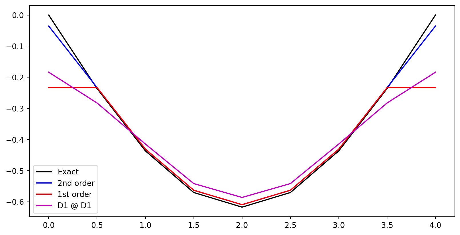
Test the accuracy of \(D^{(2)}\), \(D^{(2)}\) with only first order boundary and \(D^{(1)}D^{(1)}\)
The main advantage of using difference matrices is that they make it easy to solve equations
- Discretize \(\rightarrow\) Simply replace \(k\)’th derivative in the ODE with the \(k\)’th derivative matrix
- Apply boundary conditions to the assembled matrix
Consider the exponential decay model
\[ u' + au = 0, \, t \in (0, T], u(0)=I. \]
Replace derivatives with derivative matrices (\(u'=D^{(1)}\boldsymbol{u}, u = \mathbb{I}\boldsymbol{u}\)):
\[ (D^{(1)} + a \mathbb{I})\boldsymbol{u} = \boldsymbol{0}, \]
where \(\mathbb{I} \in \mathbb{R}^{N+1\times N+1}\) is the identity matrix and \(\boldsymbol{0}\in \mathbb{R}^{N+1}\) is a null-vector. We get
\[ A \boldsymbol{u} = \boldsymbol{0}, \quad A = D^{(1)}+a\mathbb{I} \]
which is trivially solved to \(\boldsymbol{u}=\boldsymbol{0}\) before adding boundary conditions. Not after.
Apply boundary condition by modifying both the coefficient matrix \(A\) and the rhs vector \(\boldsymbol{b}\)
With just the derivative matrix we have the problem
\[ A \boldsymbol{u} = \boldsymbol{b}, \quad \text{for} \quad \boldsymbol{b}\in \mathbb{R}^{N+1} \]
\[ \small \underbrace{ \frac{1}{2h} \begin{bmatrix} -3+2ah & 4 & -1 & 0 & 0 & 0 & 0 & 0 \\ -1 & 2ah & 1 & 0 & 0 & 0 & 0 & \cdots \\ 0 & -1 & 2ah & 1 & 0 & 0 & 0 & \cdots \\ \vdots & & & \ddots & & & &\cdots \\ \vdots & 0 & 0 & 0 & -1& 2ah& 1& 0 \\ \vdots & 0 & 0& 0& 0& -1& -2ah& 1 \\ 0 & 0 & 0 & 0 & 0 & 1 & -4 & 3+2ah \end{bmatrix} }_{D^{(1)}+a\mathbb{I}} \underbrace{\begin{bmatrix} u^0 \\ u^1 \\ u^2 \\ \vdots \\ u^{N-2} \\ u^{N-1} \\ u^{N} \end{bmatrix}}_{\boldsymbol{u}} = \underbrace{ \begin{bmatrix} b^0 \\ b^1 \\ b^2 \\ \vdots \\ b^{N-2} \\ b^{N-1} \\ b^{N} \\ \end{bmatrix}}_{\boldsymbol{b}} = \]
In order to enforce that \(u(0)= u^0 = I\), we can modify the first row of the coefficient matrix \(A\) and the right hand side vector \(\boldsymbol{b}\)
Modify \(A\) and \(\boldsymbol{b}\) to enforce boundary conditions
\[ \small \underbrace{ \frac{1}{2h} \begin{bmatrix} 2h & 0 & 0 & 0 & 0 & 0 & 0 & 0 \\ -1 & 2ah & 1 & 0 & 0 & 0 & 0 & \cdots \\ 0 & -1 & 2ah & 1 & 0 & 0 & 0 & \cdots \\ \vdots & & & \ddots & & & &\cdots \\ \vdots & 0 & 0 & 0 & -1& 2ah& 1& 0 \\ \vdots & 0 & 0& 0& 0& -1& -2ah& 1 \\ 0 & 0 & 0 & 0 & 0 & 1 & -4 & 3+2ah \end{bmatrix} }_{A} \underbrace{\begin{bmatrix} u^0 \\ u^1 \\ u^2 \\ \vdots \\ u^{N-2} \\ u^{N-1} \\ u^{N} \end{bmatrix}}_{\boldsymbol{u}} = \underbrace{ \begin{bmatrix} I \\ 0 \\ 0 \\ \vdots \\ 0 \\ 0 \\ 0 \\ \end{bmatrix}}_{\boldsymbol{b}} \]
Now the equation in the first row states that \(u^0 = I\), whereas the remaining rows are unchanged and solve the central and implicit problem for row \(n\) (row \(N\) is slightly different)
\[ \frac{u^{n+1}-u^{n-1}}{2h} + au^n = 0 \]
Implement decay problem
N = 10
dt = 0.5
a = 5
T = N*dt
t = np.linspace(0, N*dt, N+1)
D1 = sparse.diags([-1, 1], np.array([-1, 1]), (N+1, N+1), 'lil')
D1[0, :3] = -3, 4, -1
D1[-1, -3:] = 1, -4, 3
D1 *= (1/(2*dt))
Id = sparse.eye(N+1)
A = D1 + a*Id
b = np.zeros(N+1)
b[0] = I
A[0, :3] = 1, 0, 0 # boundary condition
A.toarray()
array([[ 1., 0., 0., 0., 0., 0., 0., 0., 0., 0., 0.],
[-1., 5., 1., 0., 0., 0., 0., 0., 0., 0., 0.],
[ 0., -1., 5., 1., 0., 0., 0., 0., 0., 0., 0.],
[ 0., 0., -1., 5., 1., 0., 0., 0., 0., 0., 0.],
[ 0., 0., 0., -1., 5., 1., 0., 0., 0., 0., 0.],
[ 0., 0., 0., 0., -1., 5., 1., 0., 0., 0., 0.],
[ 0., 0., 0., 0., 0., -1., 5., 1., 0., 0., 0.],
[ 0., 0., 0., 0., 0., 0., -1., 5., 1., 0., 0.],
[ 0., 0., 0., 0., 0., 0., 0., -1., 5., 1., 0.],
[ 0., 0., 0., 0., 0., 0., 0., 0., -1., 5., 1.],
[ 0., 0., 0., 0., 0., 0., 0., 0., 1., -4., 8.]])Compare with exact solution
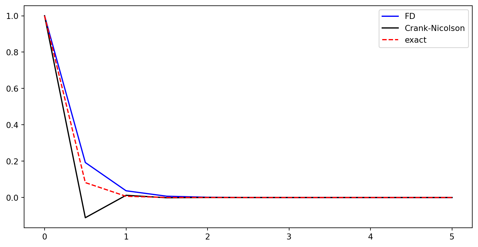
The accuracy is similar to the Crank-Nicolson method discussed in lectures 1-2. However, the FD method is not a recursive marching method, since the equation for \(u^n\) depends on the solution at \(u^{n+1}\)! This implicit FD method is unconditionally stable. Normally, only marching methods are analysed for stability.
The vibration eq. is often considered as a BVP
\[ u''(t) + \omega^2 u(t) = 0, \quad u(0) = u(T) = I, \quad t=(0, T) \]
Discretize by replacing the derivative with a second differentiation matrix
\[ (D^{(2)} + \omega^2 \mathbb{I}) \boldsymbol{u} = \boldsymbol{b} \]
w = 2*np.pi
T, N, I = 3., 35, 1.
dt = T/N
D2 = sparse.diags([1, -2, 1], np.array([-1, 0, 1]), (N+1, N+1), 'lil')
D2 *= (1/(dt**2)) # never mind the edges n=0 or n=N because these rows will be overwritten
Id = sparse.eye(N+1)
A = D2 + w**2*Id
b = np.zeros(N+1)
A.toarray()*dt**2
array([[-1.71, 1. , 0. , ..., 0. , 0. , 0. ],
[ 1. , -1.71, 1. , ..., 0. , 0. , 0. ],
[ 0. , 1. , -1.71, ..., 0. , 0. , 0. ],
...,
[ 0. , 0. , 0. , ..., -1.71, 1. , 0. ],
[ 0. , 0. , 0. , ..., 1. , -1.71, 1. ],
[ 0. , 0. , 0. , ..., 0. , 1. , -1.71]], shape=(36, 36))Apply boundary conditions to the first and last rows
\[ \begin{align} u^0 &= I \\ u^N &= I \end{align} \]
array([[   1.   ,    0.   ,    0.   , ...,    0.   ,    0.   ,    0.   ],
       [ 136.111, -232.744,  136.111, ...,    0.   ,    0.   ,    0.   ],
       [   0.   ,  136.111, -232.744, ...,    0.   ,    0.   ,    0.   ],
       ...,
       [   0.   ,    0.   ,    0.   , ..., -232.744,  136.111,    0.   ],
       [   0.   ,    0.   ,    0.   , ...,  136.111, -232.744,  136.111],
       [   0.   ,    0.   ,    0.   , ...,    0.   ,    0.   ,    1.   ]],
      shape=(36, 36))
Solve the vibration equation
Generic finite difference stencils
We have seen that it is quite simple to develop finite difference stencils for any derivative, using either forward or backward points. Can this be generalized?
Yes! Of course it can. The generic Taylor expansion around \(x=x_0\) reads
\[ u(x) = \sum_{i=0}^{M} \frac{(x-x_0)^i}{i!} u^{(i)}(x_0) + \mathcal{O}((x-x_0)^{M}), \]
where \(u^{(i)}(x_0) = \frac{d^{i}u}{dx^{i}}|_{x=x_0}\) and the are \(M+1\) terms in the expansion.
Use only \(x=x_0+ph\), where \(p\) is an integer and \(h\) is a constant (\(\Delta t\) or \(\Delta x\))
\[ u^{n+p} = \sum_{i=0}^{M} \frac{(ph)^i}{i!} u^{(i)}(x_0) + \mathcal{O}(h^{M+1}), \]
where \(u^{n+p} = u(x_0+ph)\)
Generic FD
The truncated Taylor expansions for a given \(p\) can be written \[ u^{n+p} = \sum_{i=0}^{M} \frac{(ph)^i}{i!} u^{(i)}(x_0) = \sum_{i=0}^{M} c_{pi} du_i \]
using \(c_{pi} = \frac{(ph)^i}{i!}\) and \(du_i = u^{(i)}(x_0)\).
This can be understood as a matrix-vector product
\[ \boldsymbol{u} = C \boldsymbol{du}, \]
where \(\boldsymbol{u} = (u^{n+p})_{p=p_0}^{M+p_0}\), \(C = (c_{p_0+p,i})_{p,i=0}^{M,M}\) and \(\boldsymbol{du}=(du_i)_{i=0}^M\). Here \(p_0\) is an integer representing the lowest value of \(p\) in the stencil.
For \(p_0=-2\) and \(M=4\):
\[ \boldsymbol{u} = (u^{n-2}, u^{n-1}, u^{n}, u^{n+1}, u^{n+2})^T \quad \boldsymbol{du} =(u^{(0)}, u^{(1)}, u^{(2)}, u^{(3)}, u^{(4)})^T \]
The stencil matrix
For \(p_0=-2\) and \(M=4\) we get 5 Taylor expansions
\[ \begin{align*} u^{n-2} &= \sum_{i=0}^{M} \frac{(-2h)^i}{i!} du_i \\ u^{n-1} &= \sum_{i=0}^{M} \frac{(-h)^i}{i!} du_i \\ u^{n} &= du_0 \\ u^{n+1} &= \sum_{i=0}^{M} \frac{(h)^i}{i!} du_i \\ u^{n+2} &= \sum_{i=0}^{M} \frac{(2h)^i}{i!} du_i \\ \end{align*} \]
The stencil matrix ctd
Expanding the sums these 5 Taylor expansions can be written in matrix form
\[ \small \underbrace{ \begin{bmatrix} u^{n-2}\\ u^{n-1}\\ u^{n}\\ u^{n+1}\\ u^{n+2}\\ \end{bmatrix}}_{\boldsymbol{u}} = \underbrace{\begin{bmatrix} \frac{(-2h)^0}{0!} & \frac{(-2h)^1}{1!} & \frac{(-2h)^2}{2!} & \frac{(-2h)^3}{3!} & \frac{(-2h)^4}{4!} \\ \frac{(-h)^0}{0!} & \frac{(-h)^1}{1!} & \frac{(-h)^2}{2!} & \frac{(-h)^3}{3!} & \frac{(-h)^4}{4!} \\ 1 & 0 & 0 & 0 & 0 \\ \frac{(h)^0}{0!} & \frac{(h)^1}{1!} & \frac{(h)^2}{2!} & \frac{(h)^3}{3!} & \frac{(h)^4}{4!} \\ \frac{(2h)^0}{0!} & \frac{(2h)^1}{1!} & \frac{(2h)^2}{2!} & \frac{(2h)^3}{3!} & \frac{(2h)^4}{4!} \\ \end{bmatrix}}_{C} \underbrace{ \begin{bmatrix} du_{0} \\ du_1 \\ du_2 \\ du_3 \\ du_4 \end{bmatrix}}_{\boldsymbol{du}} \]
\[ \boldsymbol{u} = C \boldsymbol{du} \]
Invert to obtain
\[ \boldsymbol{du} = C^{-1} \boldsymbol{u} \]
Since \(du_i\) is an approximation to the i’th derivative we can now compute any derivative stencil!
Second order 2nd derivative stencil
We have been using the following stencil
\[ du_2 = u^{(2)}(x_0) = \frac{u^{n+1}-2u^n+u^{n-1}}{h^2}. \]
Let’s derive this with the approach above. The scheme is central and second order so we use \(p_0=-1\) and \(M=2\) (hence \(p=(-1, 0, 1)\)). Insert into the recipe for \(C\)
\[ C = \begin{bmatrix} 1 & -h & \frac{h^2}{2} \\ 1 & 0 & 0 \\ 1 & h & \frac{h^2}{2} \end{bmatrix} \]
In Sympy
Print \(C\) matrix
The last row in \(C^{-1}\) represents \(u''\)! The middle row represents a second order central \(u'\).
Create a vector for \(\boldsymbol{u}\) and print \(u'\) and \(u''\)
We can get any stencil
Create a function that computes \(C\) for any \(p_0\) and \(M\)
\(p_0=-1, M=2\)
\(\displaystyle \left[\begin{matrix}1 & - h & \frac{h^{2}}{2}\\1 & 0 & 0\\1 & h & \frac{h^{2}}{2}\end{matrix}\right]\)
A central stencil of order \(l\) for the \(k\)’th’ derivative requires \(M+1\) points, where
\[ M = l + 2 \left\lfloor \frac{k-1}{2} \right\rfloor \]
Forward and backward
Non-central schemes requires one more point for the same accuracy as central
Forward \(u''\)
\(p_0=0, M=3\)
\(\displaystyle \left[\begin{matrix}1 & 0 & 0 & 0\\- \frac{11}{6 h} & \frac{3}{h} & - \frac{3}{2 h} & \frac{1}{3 h}\\\frac{2}{h^{2}} & - \frac{5}{h^{2}} & \frac{4}{h^{2}} & - \frac{1}{h^{2}}\\- \frac{1}{h^{3}} & \frac{3}{h^{3}} & - \frac{3}{h^{3}} & \frac{1}{h^{3}}\end{matrix}\right]\)
Backward \(u''\)
\(p_0 = -3, M=3\)
\(\displaystyle \left[\begin{matrix}0 & 0 & 0 & 1\\- \frac{1}{3 h} & \frac{3}{2 h} & - \frac{3}{h} & \frac{11}{6 h}\\- \frac{1}{h^{2}} & \frac{4}{h^{2}} & - \frac{5}{h^{2}} & \frac{2}{h^{2}}\\- \frac{1}{h^{3}} & \frac{3}{h^{3}} & - \frac{3}{h^{3}} & \frac{1}{h^{3}}\end{matrix}\right]\)
Recognize the third row in the forward scheme:
\[ u'' = \frac{-u^{n+3} + 4u^{n+2} - 5u^{n+1} +2 u^{n}}{h^2} \]
Fourth order central \(\small p_0=-2, M=4\)
\(\displaystyle \left[\begin{matrix}0 & 0 & 1 & 0 & 0\\\frac{1}{12 h} & - \frac{2}{3 h} & 0 & \frac{2}{3 h} & - \frac{1}{12 h}\\- \frac{1}{12 h^{2}} & \frac{4}{3 h^{2}} & - \frac{5}{2 h^{2}} & \frac{4}{3 h^{2}} & - \frac{1}{12 h^{2}}\\- \frac{1}{2 h^{3}} & \frac{1}{h^{3}} & 0 & - \frac{1}{h^{3}} & \frac{1}{2 h^{3}}\\\frac{1}{h^{4}} & - \frac{4}{h^{4}} & \frac{6}{h^{4}} & - \frac{4}{h^{4}} & \frac{1}{h^{4}}\end{matrix}\right]\)
Third row gives us:
\[ u'' = \frac{-u^{n+2} + 16u^{n+1} - 30 u^n + 16 u^{n-1} - u^{n-2}}{12 h^2} + \mathcal{O}(h^4) \]
where the order \(l = M - 2 \left\lfloor \frac{2-1}{2} \right \rfloor = M = 4\).
What is the order of the fourth derivative \(u''''=\frac{u^{n+2}-4u^{n+1}+6u^{n}-4u^{n-1}+u^{n-2}}{h^4}\)?
\(l = M - 2 \left\lfloor \frac{4-1}{2} \right \rfloor = M - 2 = 2\)